Excitation energies at the SCF-level

In this tutorial we will look at the theory behind the calculation of excitation energies at the SCF-level, that is, either by time-dependent Hartree-Fock (TD-HF) or TD-DFT. The implementations in DIRAC are presented in [Bast2009].

Excitation energies ${\omega }_m$ are found by solving the generalized eigenvalue problem

$$(E_0^{[2]}-\hslash \lambda S^{[2]})X_m=0;(1)$$

where the matrices $E_0^{[2]}$ and $S^{[2]}$ are the electronic Hessian and generalized metric, respectively. From their structure, it can be shown that solution vectors come in pairs

$$\begin{array}{r}{\lambda }_{+;n}=+\left|{\omega }_n\right|,{\mathit{X}}_{+;n}=\left[\begin{array}{c}{\mathit{Z}}_n\\ {\mathit{Y}}_n^{\ast }\end{array}\right],{\lambda }_{-;n}=-\left|{\omega }_n\right|,{\mathit{X}}_{-;n}=\left[\begin{array}{c}{\mathit{Y}}_n\\ {\mathit{Z}}_n^{\ast }\end{array}\right].\end{array}$$

Transition moments associated with operator ${\hat{h}}_A$ for transitions $n\leftarrow 0$ are generally calculated as

$$⟨n|{\hat{h}}_A|0⟩={\mathit{X}}_{+;n}^{†}{\mathit{E}}_A^{[1]};(2)$$

where appears solution vector ${\mathit{X}}_{+;n}^{†}$ and property gradient ${\mathit{E}}_A^{[1]}$. The property gradient is given by

$$\begin{array}{r}{\mathit{E}}_B^{[1]}=\left[\begin{array}{c}{\mathit{g}}_B\\ {\mathrm{\Theta }}_{hB}{\mathit{g}}_B^{\ast }\end{array}\right];g_{B;ai}=-h_{B;ai}.\end{array}$$

An important generalization above is that, in addition to Hermitian operators ${\hat{h}}_B$ (${\mathrm{\Theta }}_{hB}=+1$), imposed by the tenets of quantum mechanics, we also allow anti-Hermitian ones (${\mathrm{\Theta }}_{hB}=-1$).

A key to computational efficiency is to consider a decomposition of solution vectors in terms of components of well-defined Hermiticity and time reversal symmetry. Using a pair of solution vectors ${\mathit{X}}_{+}$ and ${\mathit{X}}_{-}$, we may form Hermitian and anti-Hermitian combinations

$$\begin{array}{r}\begin{array}{lcl}{\mathit{X}}_h& =& \frac{1}{2}({\mathit{X}}_{+}+{\mathit{X}}_{-})=\left[\begin{array}{c}\mathit{Z}+\mathit{Y}\\ {\mathit{Y}}^{\ast }+{\mathit{Z}}^{\ast }\end{array}\right]=\left[\begin{array}{c}\mathit{h}\\ {\mathit{h}}^{\ast }\end{array}\right]\\ {\mathit{X}}_a& =& \frac{1}{2}({\mathit{X}}_{+}-{\mathit{X}}_{-})=\left[\begin{array}{c}\mathit{Z}-\mathit{Y}\\ {\mathit{Y}}^{\ast }-{\mathit{Z}}^{\ast }\end{array}\right]=\left[\begin{array}{c}\mathit{a}\\ -{\mathit{a}}^{\ast }\end{array}\right].\end{array}\end{array}$$

The inverse relations therefore provide a separation of solution vectors into Hermitian and anti-Hermitian contributions

$${\mathit{X}}_{+}={\mathit{X}}_h+{\mathit{X}}_a;{\mathit{X}}_{-}={\mathit{X}}_h-{\mathit{X}}_a.$$

Further decomposition of each contribution into time-symmetric and time-antisymmetric parts give vectors that are well-defined with respect to both Hermiticity and time reversal symmetry

$${\mathit{U}}^{†}({\mathrm{\Theta }}_h,{\mathrm{\Theta }}_t)=\left[\begin{array}{cccccccc}{\mathit{c}}^{†}& {\mathit{d}}^{†}& {\mathrm{\Theta }}_t{\mathit{c}}^T& {\mathrm{\Theta }}_t{\mathit{d}}^T& {\mathrm{\Theta }}_h{\mathit{c}}^T& {\mathrm{\Theta }}_h{\mathit{d}}^T& {\mathrm{\Theta }}_h{\mathrm{\Theta }}_t{\mathit{c}}^{†}& {\mathrm{\Theta }}_h{\mathrm{\Theta }}_t{\mathit{d}}^{†}\end{array}\right]$$

where

$$c_{ai}=x_{ai}\text{and}{d}_{ai}=x_{a\bar{i}}$$

and the index overbar refers to a Kramers’ partner in a Kramers-restricted orbital set. The scalar product of such vectors is given by [Saue2002a]

$${\mathit{U}}_1^{†}({\mathrm{\Theta }}_{h1},{\mathrm{\Theta }}_{t1}){\mathit{U}}_2({\mathrm{\Theta }}_{h2},{\mathrm{\Theta }}_{t2})=(1+{\mathrm{\Theta }}_{h1}{\mathrm{\Theta }}_{h2}{\mathrm{\Theta }}_{t1}{\mathrm{\Theta }}_{t2})[z+{\mathrm{\Theta }}_{h1}{\mathrm{\Theta }}_{h2}{z}^{\ast }];z=({\mathit{c}}_1^{†}{\mathit{c}}_2+{\mathit{d}}_1^{†}{\mathit{d}}_2),$$

and one may therefore distinguish three cases

$$\begin{array}{r}{\mathit{U}}_1^{†}({\mathrm{\Theta }}_{h1},{\mathrm{\Theta }}_{t1}){\mathit{U}}_2({\mathrm{\Theta }}_{h2},{\mathrm{\Theta }}_{t2})=\{\begin{array}{ll}0& ;{\mathrm{\Theta }}_{h1}{\mathrm{\Theta }}_{h2}=-{\mathrm{\Theta }}_{t1}{\mathrm{\Theta }}_{t2}\\ 4Re\left[z\right]& ;{\mathrm{\Theta }}_{h1}{\mathrm{\Theta }}_{h2}={\mathrm{\Theta }}_{t1}{\mathrm{\Theta }}_{t2}=+1\\ 4iIm\left[z\right]& ;{\mathrm{\Theta }}_{h1}{\mathrm{\Theta }}_{h2}={\mathrm{\Theta }}_{t1}{\mathrm{\Theta }}_{t2}=-1\end{array}.(3)\end{array}$$

One may show that Hermiticity is conserved when multiplying such a trial vector by the electronic Hessian, whereas it is reversed by the generalized metric. However, both the electronic Hessian and the generalized metric conserves time reversal symmetry. The implication is that the time-symmetric and time-antisymmetric components of a solution vector does not mix upon solving the generalized eigenvalue problem, and one can dispense with one of them. From a physical point of view, this can be understood from the observation that excited states can be reached through both time-symmetric and time-antisymmetric operators. In order to employ the quaternion symmetry scheme, we choose to work with the time-symmetric vectors. It follows from the above that their scalar product are either zero or real. In practice, a property gradient is therefore always contracted with the component of the solution vector having the same hermiticity, so that all transition moments are real.

Practical example

We consider the excitation $1s_{1/2}\to 3p_{3/2}(\left|m_j\right|=1/2)$ of the magnesium atom. We limit attention to boson irrep $B_{1u}$, corresponding to the symmetry of the $z$ - coordinate (${\mathrm{\Gamma }}_z$). We work within the electric dipole approximation and from a character table of $D_{2h}$ it is clear that we will only get non-zero transition moments from the z-component of the electric dipole operator.

We start from the menu file ed.inp

**DIRAC                                                                                             
.WAVE FUNCTION                                                                                      
.ANALYZE                                                                                            
.PROPERTIES                                                                                         
**INTEGRALS                                                                                         
*READIN                                                                                             
.UNCONT                                                                                             
**WAVE FUNCTION                                                                                     
.SCF                                                                                                
*SCF                                                                                                
.CLOSED SHELL                                                                                       
6 6                                                                                                 
**PROPERTIES                                                                                        
*EXCITATION ENERGIES                                                                                
.PRINT                                                                                              
10                                                                                                  
.OCCUP                                                                                              
1                                                                                                   
                                                                                                    
.VIRTUAL                                                                                            
                                                                                                    
6                                                                                                   
.ANALYZE                                                                                            
! Excitations s -> p                                                                                
.EXCITATION ! B1u                                                                                   
5 1                                                                                                 
**ANALYZE                                                                                           
.MULPOP                                                                                             
*MULPOP                                                                                             
.VECPOP                                                                                             
1..oo                                                                                               
1..oo                                                                                               
**MOLECULE                                                                                          
*BASIS                                                                                              
.DEFAULT                                                                                            
dyall.ae2z                                                                                          
**END OF                                                                                            

and the xyz-file Mg.xyz

1                                                                                                   
                                                                                                    
Mg  0.0D0 0.0D0 0.0D0                                                                              

and run our calculation using:

pam --inp=ed --mol=Mg.xyz --get "DFCOEF PAMXVC"

We are keeping some file for later use, see below. It can be seen in the menu file ed.inp that excitations are only allowed from the first gerade orbital ($1s_{1/2}$) to the sixth ungerade one ($3p_{3/2,1/2}$). The nature of these orbitals can be seen from the Mulliken population analysis in the output.

We have increased the print level significantly in order to be able to look a bit under the hood. Let us first look at the property gradient

$$g_{ai}\to -⟨3p_{3/2;1/2}|{\hat{\mu }}_z|1s_{1/2;+1/2}⟩;g_{a\bar{i}}\to -⟨3p_{3/2;1/2}|{\hat{\mu }}_z|1s_{1/2;-1/2}⟩;{\hat{\mu }}_z=-ez.$$

The matrix element $g_{ai}$ may be written as

$$g_{ai}=-\int {\mathrm{\Omega }}_{ai}\left(\mathit{r}\right){\hat{\mu }}_z\left(\mathit{r}\right)d^3\mathit{r};{\mathrm{\Omega }}_{ai}\left(\mathit{r}\right)={\varphi }_a^{†}\left(\mathit{r}\right){\varphi }_i\left(\mathit{r}\right)$$

and similar for $g_{a\bar{i}}$. For present purposes it suffices to think in terms of 2-component spinors. Since $s_{1/2}$ and $p_{3/2}$ have opposite parity, they will in the conventions of DIRAC have different symmetry structures

$$\begin{array}{r}{s}_{1/2}\to \left[\begin{array}{c}({\mathrm{\Gamma }}_0,{\mathrm{\Gamma }}_{R_z})\\ ({\mathrm{\Gamma }}_{R_y},{\mathrm{\Gamma }}_{R_x})\end{array}\right];p_{3/2}\to \left[\begin{array}{c}({\mathrm{\Gamma }}_{xyz},{\mathrm{\Gamma }}_z)\\ ({\mathrm{\Gamma }}_y,{\mathrm{\Gamma }}_x)\end{array}\right].\end{array}$$

In addition we have to remember the relation between Kramers partners

$$\begin{array}{r}\varphi =\left[\begin{array}{c}{\varphi }^{\alpha }\\ {\varphi }^{\beta }\end{array}\right];\bar{\varphi }=\left[\begin{array}{c}-{\varphi }^{\beta \ast }\\ {\varphi }^{\alpha \ast }\end{array}\right].\end{array}$$

In terms of symmetry the orbital distributions are

$${\mathrm{\Omega }}_{(p_{3/2};s_{1/2})}=({\mathrm{\Gamma }}_{xyz},{\mathrm{\Gamma }}_z);{\mathrm{\Omega }}_{(p_{3/2};\overline{s_{1/2}})}=({\mathrm{\Gamma }}_y,{\mathrm{\Gamma }}_x).$$

In the present case the operator symmetry is ${\mathrm{\Gamma }}_z$. Since the integrand of the matrix element has to be totally symmetric, we see that only the imaginary part of $g_{ai}$ will be non-zero; the partner element $g_{a\bar{i}}$ is strictly zero. The generally complex gradient elements are combined into a quaternion one

$${}^Q{g}_{AI}=g_{ai}+g_{a\bar{i}}\check{j}$$

and, indeed, when we look in the output we find

                                Output from GPGET
                                -----------------

* Gradient (e-e) of property EpolL01X00Y00Z01

*** A imag part ***; NROW,NCOL,LRQ,LCQ:   1   1   1   1


               Column   1
       1      -0.00682451
    ==== End of matrix output ====

Here the notation EpolLnlXnxYnyZnz refers to a Cartesian electric multipole operator ${\hat{Q}}^{[nl]}=-e{x}^{nx}{y}^{ny}{z}^{nz};nx+ny+nz=nl$. Since this is a time symmetric, Hermitian operator, it will be contracted with the Hermitian part of the solution vector. In this particular case we have only a single orbital rotation, and between two orbitals of positive energy, so the relevant part of the solution vector is

 E+ part of solution vectors for  1 excitations:
* Vector nr.    1

*** A imag part ***; NROW,NCOL,LRQ,LCQ:   1   1   1   1


               Column   1
       1       0.35355084
    ==== End of matrix output ====

Searching in the output, we find the corresponding calculated transition moment

< 0 |EpolL01X00Y00Z01|  1 > = -4.8256194928E-03 a.u.,

which is easily seen to be $2\ast 0.35355084\ast -0.00682451$. (With respect to Eq.(3) a factor two seems to be missing; this is appears to be connected to the scaling of eigenvectors in subroutine XPPORD.)

We may proceed to visualize the transition moment density

$$T(\mathit{r})=-\sum _{ai}{x}_{+;n;ai}^{\ast }{\mathrm{\Omega }}_{ai}\left(\mathit{r}\right){\hat{\mu }}_z\left(\mathit{r}\right)$$

as a radial distribution, that is

$$T(r)={\int }_0^{2\pi }{\int }_0^{\pi }T(\mathbf{r})r^2\sin \theta d\theta d\varphi$$

As preparation we first inspect the file PAMXVC of solution vectors

dirac 2074>rspread.x PAMXVC

 Solution vectors found on file : PAMXVC

** Solution vector : PP EXCITATIONB1u Irrep:   5 Trev:   1
  1 Type : E+ Freq.:    48.935572 Rnorm:   0.16E-13 Length:         1
  2 Type : E- Freq.:    48.935572 Rnorm:   0.16E-13 Length:         1

We see that the Hermitian e-e part of the solution vector E+ is the first vector on the file, which therefore leads us to set up the input file length.inp as

**DIRAC
.PROPERTIES
**INTEGRALS
*READIN
.UNCONT
**WAVE FUNCTION
.SCF
*SCF
.CLOSED SHELL
6 6
**GRID
.ULTRAFINE
**PROPERTIES
*EXPECTATION VALUES
.ORBANA
.OPERATOR
 'XXSECMOM'
.OPERATOR
 'YYSECMOM'
.OPERATOR
 'ZZSECMOM'
**VISUAL
.EDIPZ
 PAMXVC 1
.RADIAL
0.0D0 0.0D0 0.0D0
10.0
500
.3D_INT
**MOLECULE
*BASIS
.DEFAULT
dyall.ae2z
**END OF

We now generate the radial distribution using:

pam --inp=length --mol=Mg.xyz --put "DFCOEF PAMXVC" --get "plot.radial.scalar=length.dat"

First we may note at the end of the output

   The radial distribution integrates to:    4.8280356220858738E-003

and so we see that the radial distribution integrates to the value obtained in our previous calculation.

Next, with a suitable plotting program (I used xmgrace) we can visualize the radial distribution

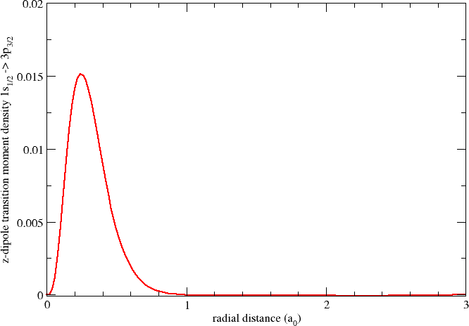
To get some idea of the extent of the z-electric dipole moment transition density associated with the $1s_{1/2}\to 3p_{3/2}(\left|m_j\right|=1/2)$ transition, I have included in the input the calculation of orbital sizes as $<r^2{>}^{1/2}={(<x^2>+<y^2>+<z^2>)}^{1/2}$. Extracting and using the data from the output I obtain the following table (orbital labels are taken from the Mulliken analysis of the first calculation):

Sym.	Orb.	$<x^2>$	$<y^2>$	$<z^2>$	$<r^2{>}^{1/2}$
E1g	1s 1/2; 1/2	0.008	0.008	0.008	0.151
E1g	2s 1/2; 1/2	0.190	0.190	0.190	0.754
E1g	3s 1/2; 1/2	4.106	4.106	4.106	3.510
E1u	2p 1/2; 1/2	0.198	0.198	0.198	0.772
E1u	2p 3/2; -3/2	0.240	0.240	0.120	0.774
E1u	3p 3/2; 1/2	0.160	0.160	0.279	0.774

We see that the radial distribution peaks around 0.25 $a_0$ which is slightly outside the size of the $1s_{1/2}$ orbital.