Full scope application of POLPRP to an osmium carbonyl complex
In this second section we describe a toolchain how to arrive at physically meaningful spectra suitable for comparison to experiment and publication. This toolchain emerged over the years of application of propagator code and has proven to be useful. Shortly, we will combine the individual small helpers to a combined postprocessing module written in Python3 bringing about a lot of simplification.
The excitation spectrum of the osmium complex exhibits sizeable differences between a scalar relativistic and a four-component treatment. By this we extract the effect of pure spin-orbit coupling on the spectrum.
Therefore two individual calculations once with the .SPINFREE and the .X2Cmmf Hamiltonian are necessary. Since the postprocessing steps are identical for both pathways we do not need to repeat it. The molecule and X2Cmmf input read as
INTGRL
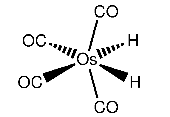
H2 Os (CO) 4 complex, C2v symmetry
cc-pVTZ basis
C 4 A
76. 1
Os 0.00000000 0.00000000 0.00000000
LARGE BASIS dyall.v3z
8. 4
O 2.41214315 0.00000000 -1.98152075
O -2.41214315 0.00000000 -1.98152075
O -0.00000000 -3.03655487 0.59571453
O -0.00000000 3.03655487 0.59571453
LARGE BASIS cc-pVTZ
6. 4
C -0.00000000 -1.93462292 0.31819191
C -0.00000000 1.93462292 0.31819191
C 1.51252482 0.00000000 -1.28284746
C -1.51252482 0.00000000 -1.28284746
LARGE BASIS cc-pVTZ
1. 2
H 1.10331142 0.00000000 1.25671302
H -1.10331142 0.00000000 1.25671302
LARGE BASIS cc-pVTZ
FINISH
**DIRAC
.WAVE FUNCTION
.ANALYZE
**GENERAL
**HAMILTONIAN
.X2Cmmf
**INTEGRALS
*READIN
.UNCONT
**WAVE FUNCTION
.SCF
.POLPRP
*SCF
.CLOSED SHELL
 134
**ANALYZE
.MULPOP
*MULPOP
.VECPOP
 all
.LABDEF
 28
C_d         105,106,107,108,116,117,154,155,163,164,165
C_d         166,200,201,207,208,44,45,46,47,57,58,59
C_d         60
C_f         109,110,111,112,113,114,118,119,120,121,156
C_f         157,158,159,167,168,169,170,171,172,202,203
C_f         204,205,209,210,211,212,48,49,50,51,52,53
C_f         61,62,63,64,65,66
C_p         103,104,115,153,161,162,199,206,42,43,55
C_p         56
C_s         102,160,41,54
H_d         123,124,176,177,178,179,214,215,70,71,72
H_d         73
H_p         122,174,175,213,68,69
H_s         173,67
O_d         136,137,138,139,147,148,18,186,187,19,193
O_d         194,20,21,31,32,33,34,83,84,92,93,94,95
O_f         100,101,140,141,142,143,144,145,149,150,151
O_f         152,188,189,190,191,195,196,197,198,22,23
O_f         24,25,26,27,35,36,37,38,39,40,85,86,87,88
O_f         96,97,98,99
O_p         134,135,146,16,17,185,192,29,30,82,90,91
O_s         133,15,28,89
Os_d        126,180,3,4,5,75
Os_f        127,128,129,181,6,7,76,77,78,8
Os_g        10,11,12,13,130,131,132,14,182,183,184,79
Os_g        80,81,9
Os_p        125,2,74
Os_s        1
**MOLTRA
.ACTIVE
energy   -0.80  1.73   0.001
.PRPTRA
*PRPTRA
.OPERATOR
 XDIPLEN
.OPERATOR
 YDIPLEN
.OPERATOR
 ZDIPLEN
**POLPRP
.DOTRMO
.PRINT
 1
**DAVIDSON
.DVROOTS
 25
.DVMAXSP
 400
.DVMAXIT
 12
.DVCONV
 1.0E-05
*END OF
As you can see in the .mol file the complex has C2v symmetry and we use basis sets from the library shipped with DIRAC. In the input file a large number of labdef labels are visible. This is necessary later on if we want to analyze the eigenstate composition in terms of atomic orbital contributions. Hereby the grouping occurs according to the angular momentum of the atomic basis functions. A further distinction is not made and would lead to an excess of information in larger systems. In order to generate the LABDEF labels we use the utility
labdefmaker
that automatically reads the:
                             GETLAB: SO-labels
                             -----------------

* Large components:  215
  1  L A1 Os s        2  L A1 Os pz       3  L A1 Os dxx      4  L A1 Os dyy      5  L A1 Os dzz      6  L A1 Os fxxz
  7  L A1 Os fyyz     8  L A1 Os fzzz     9  L A1 Os g400    10  L A1 Os g220    11  L A1 Os g202    12  L A1 Os g040
  . . . . . . . . .
section. A little disadvantage here is that the ordered LABDEF section should be available already for the Mulliken population analysis for a proper labeling of the atomic contributions. So we recommend to run DIRAC with a preliminary input just producing the GETLAB output. Application of labdefmaker produces the file “labdef” that can be included in the production input afterwards. A manual sorting and grouping of labels is out of scope for larger systems. We perform a strict ADC-2 calculation where the satellite block just consists of the diagonal of the orbital energies (see publications). Before we include the transition moments in our analysis we want to get an overview of the final state composition. Hereby the information of a Mulliken analysis, the active orbital list and the ADCSTATE.XX files are required and their information combined. This is done by the two helper programs
spimaker and excmaker
to be excuted in series. spimaker constructs an intermediate list of spinors relating the molecular and atomic basis and excmaker combines this list with the state analysis obtained by the POLPRP calculation. The resulting ‘xstates’ file then serves as the basis for the gnuplot drawing utility that generates a composition analysis of the hole and the particle space:
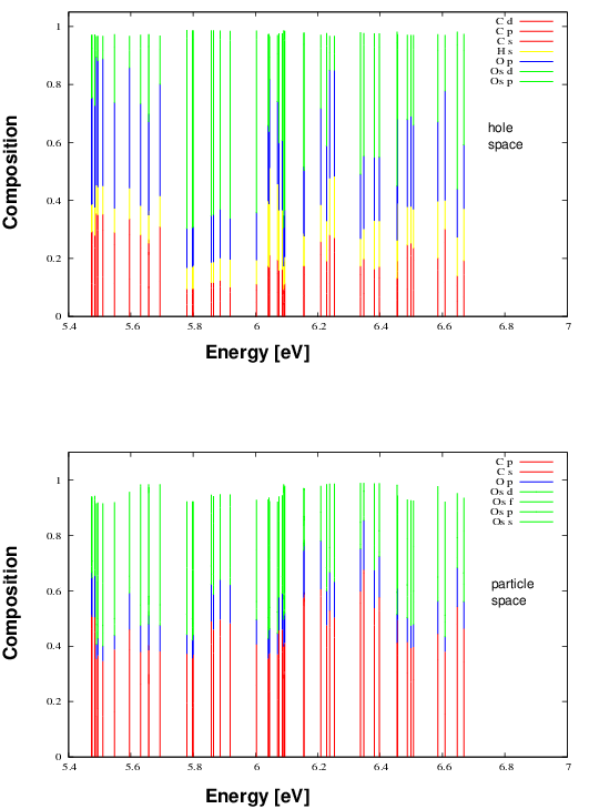
This graph shows sizeable osmium contributions in the hole and particle space being responsible for SO coupling effects in the excitation spectrum (see below).
In the next step we want to utilize the physical information provided by the transition moments. For this purpose we multiply the pole strength of the impulse peak with the oscillator strength which gives us a modulated spectrum according to the transition probability. This multiplication was done with a simple spreadsheet tool because the number of states is reasonably small. afterwards the new stick spectrum is convoluted with a Lorentzian envelope in order to account for the spectral width. This final step is performed by the
specfolder
tool. You give the number of peaks, the desired number of graphic points and the spectral width in meV. The resulting graph file can again be plotted by gnuplot and results in the following simulated spectrum:
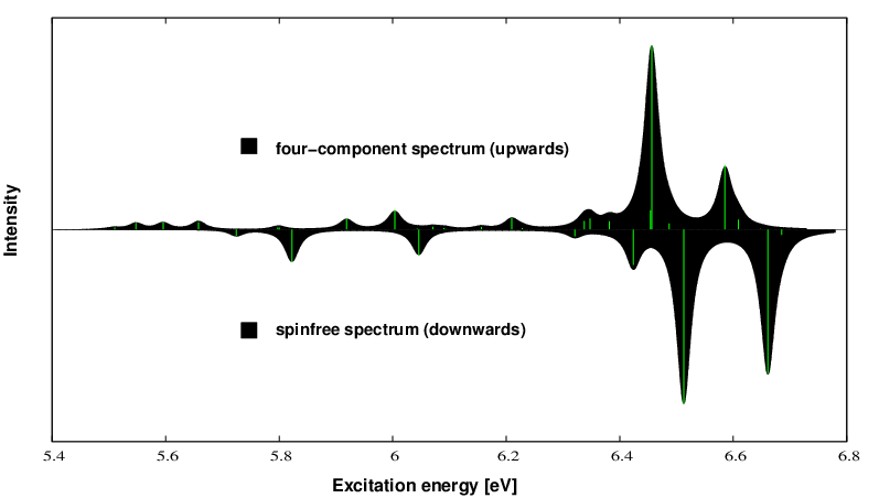
Upwards we plot the X2Cmmf spectrum, downwards the SPINFREE spectrum which exhibits the pure effect of spin-orbit coupling on the excitation spectrum. Soon an integrated python tool will come combining all the individual tasks from above.