NMR shieldings in Frozen Density Embedding (FDE) scheme with London atomic orbitals (LAOs)
In this tutorial we will show how to calculate the NMR shielding tensor with London atomic orbitals within the FDE scheme.
NMR shielding tensor in FDE scheme - theory overview
In order to calculate the NMR shielding tensor with LAOs, one must take into account modifications of the property gradient due to the use of perturbation-dependent basis sets (see [Ilias2009]). In FDE scheme, further modifications are needed, since the property gradient includes not only terms from isolated subsystems (here marked as “I” and “II”), but also a contribution from the interaction energy between these subsystems (see [Hofener2013]).
For instance, these new contributions to the property gradient of subsystem “I” can be written as (see :cite: olejniczak2017):
where \(\Omega_{pq}^{B}\) is the first-order perturbed overlap distribution, which in a basis of London orbitals consists of two terms
“direct” LAO term (the first term) and “reorthonormalization” term (in parenthesis). The \(v_{emb}^I\) is the embedding potential of subsystem I, \(w_{emb}^{I,I}\) is the embedding kernel involving subsystem I and \(w_{emb}^{I,II}\) is the embedding kernel coupling subsystem I and subsystem II.
In this tutorial we will show how to include each of these contributions to the property gradient in the calculations of the NMR shielding tensor. We will also demonstrate how to calculate and plot the first-order perturbed current density induced by magnetic field and how to use it in analysis of the NMR shielding tensor.
A sample calculation of NMR shielding tensor within FDE
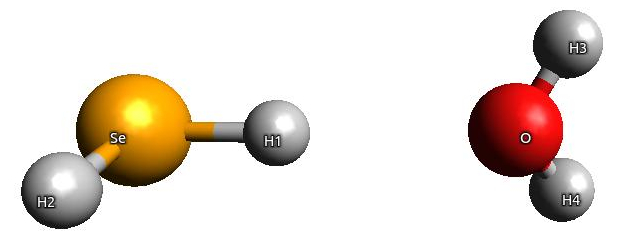
We will consider a simple system of SeH2- H2O, in which SeH2constitutes an active subsystem (subsystem I) and H2Ois an environment (subsystem II):
The computational protocol is different depending on whether the coupling between two subsystems is included or not (through the term dependent on \(w_{emb}^{I,II}\)). To avoid confusion, we will describe these two protocols separately.
We will need two molecular input files. File h2se.mol, corresponding to an active subsystem I, reads:
DIRAC


C   2    0         A
       34.    1
Se1      -0.003989   -0.034416    0.000005
LARGE BASIS cc-pVDZ
        1.    2
H2        0.089169    1.434145   -0.001364
H3        1.458406   -0.164893    0.001741
LARGE BASIS cc-pVDZ
FINISH
and file h2o.mol, standing for a subsystem II (‘environment’):
DIRAC


C   2    0         A
        1.    2
H4       -0.257088    4.261903    0.765747
H6       -0.259151    4.266296   -0.762573
LARGE BASIS cc-pVDZ
        8.    1
O5        0.036856    3.761402   -0.000251
LARGE BASIS cc-pVDZ
FINISH
In this example we will use the four-component relativistic DC Hamiltonian and DFT/LDA with small grid and small basis sets.
Calculations without the FDE coupling terms
Here we demonstrate how to include the first two terms of Eq. (1) in the property gradient: terms dependent on the embedding potential and the uncoupled embedding kernel.
In this tutorial, we use a coarse grid generated in DIRAC in preceeding calculations on SeH2- H2O ‘supermolecule’, which was then exported on a numerical_grid file. In DIRAC the numerical_grid file, which can be retrieved from DFT calculations, is divided into batches of points. However, FDE module is able to read only the continuous list of grid points, therefore such numerical_grid file has to be reformatted. This can be done by the script which can be found in utils directory of DIRAC, dft_to_fde_grid_convert.py, which should be called from the directory where the numerical_grid file is:
# make sure that the "utils/fde-mag" in DIRAC's directory is in your PATH, then:

./dft_to_fde_grid_convert.py
This script will overwrite the numerical_grid and save its original version as numerical_grid.ORIG.
Step 1: SCF calculation on the subsystem II
The first step is the calculation on subsystem II, the aim of which is to export its density and electrostatic potential on a text file.
The menu file getfrozen.inp reads:
**DIRAC
.WAVE F
**HAMILTONIAN
.DFT
 LDA
.FDE
*FDE
.EXONLY
FILEEX
.GRIDOU
GRIDOUT
.WRFRMT
TXT
**GRID
.IMPORT
numerical_grid
**INTEGRALS
.NUCMOD
1
*READIN
.UNCONTRACT
**WAVE FUNCTIONS
.SCF
*SCF
.EVCCNV
1.0E-08  1.0E-06
**ANALYZE
*END OF
and we make sure to get the text file GRIDOUT (related to the .GRIDOU keyword). We should also remember to supply two files, related to keywords .GRIDOU (GRIDOUT) and .EXONLY (FILEEX), which are copies of a numerical grid file:
cp numerical_grid GRIDOUT
cp numerical_grid FILEEX

pam --inp=getfrozen.inp --mol=h2o.mol --put="numerical_grid FILEEX GRIDOUT" --get="GRIDOUT" --outcmo

mv DFCOEF   DFCOEF.h2o
mv GRIDOUT  GRIDOUT.h2o
After this step, the GRIDOUT file will be updated: additional columns on that file correspond to the electrostatic potential and the density of subsystem II calculated in each point of a grid.
Step 2: SCF and response calculation on the subsystem I
Now we can use the information about the subsystem II written on the GRIDOUT file for constructing the embedding potential, \(v_{emb}^{I}\), and embedding kernel, \(w_{emb}^{I,I}\). In order to do that, we use the GRIDOUT file saved from Step 1 and copy it to a FROZEN file, which is given as an argument to the .FRDENS keyword.
We use the following input file for the SCF step:
**DIRAC
.WAVE F
**HAMILTONIAN
.DFT
 LDA
.FDE
*FDE
.FRDENS
FROZEN
.RDFRMT
TXT
.UPDATE
.GRIDOU
GRIDOUT
.WRFRMT
TXT
**GRID
.IMPORT
numerical_grid
**INTEGRALS
.NUCMOD
1
*READIN
.UNCONTRACT
**WAVE FUNCTIONS
.SCF
*SCF
.EVCCNV
1.0E-08  1.0E-06
*END OF
and the pam command is:
cp GRIDOUT.h2o FROZEN
cp GRIDOUT.h2o GRIDOUT

pam --inp=updatefrozen.inp --mol=h2se.mol --put="numerical_grid FROZEN GRIDOUT" --get="GRIDOUT" --outcmo

mv GRIDOUT GRIDOUT.h2se
mv DFCOEF  DFCOEF.h2se
To calculate the NMR shielding tensor, we use the following input file:
**DIRAC
.PROPERTIES
**GENERAL
.RKBIMP
**GRID
.IMPORT
numerical_grid
**HAMILTONIAN
.URKBAL
.DFT
 LDA
.FDE
*FDE
.FRDENS
FROZEN
.RDFRMT
TXT
.UPDATE
.RSP
.LAO11
**INTEGRALS
.NUCMOD
1
*READIN
.UNCONTRACT
**WAVE FUNCTIONS
.SCF
*SCF
.EVCCNV
1.0E-08  1.0E-05
**PROPERTIES
.PRINT
2
.SHIELDING
*NMR
.LONDON
.SYMCON
*LINEAR RESPONSE
.PRINT
2
.THRESH
1.0E-07
.MAXITR
100
*END OF
in which the keyword .LAO11 denotes that the contributions from the embedding potential, \(v_{emb}^{I}\), and the uncoupled embedding kernel, \(w_{emb}^{I,I}\), will be added to the property gradient. The corresponding pam command is:
cp GRIDOUT.h2o  FROZEN
cp DFCOEF.h2se  DFCOEF

pam --inp=shield_v_w11.inp --mol=h2se.mol --put="numerical_grid FROZEN" --incmo
This is the advised option. However, as the calculations of the uncoupled embedding kernel terms in the property gradient may be expensive, one may want to restrict the FDE-LAO contributions to the part dependent on the embedding potential only. In this case, the input file reads:
**DIRAC
.PROPERTIES
**GENERAL
.RKBIMP
**GRID
.IMPORT
numerical_grid
**HAMILTONIAN
.URKBAL
.DFT
 LDA
.FDE
*FDE
.FRDENS
FROZEN
.RDFRMT
TXT
.UPDATE
.RSP
.LDPT
**INTEGRALS
.NUCMOD
1
*READIN
.UNCONTRACT
**WAVE FUNCTIONS
.SCF
*SCF
.EVCCNV
1.0E-08  1.0E-05
**PROPERTIES
.PRINT
2
.SHIELDING
*NMR
.LONDON
.SYMCON
*LINEAR RESPONSE
.PRINT
2
.THRESH
1.0E-07
.MAXITR
100
*END OF
and the corresponding pam command is:
cp GRIDOUT.h2o  FROZEN
cp DFCOEF.h2se  DFCOEF

pam --inp=shield_v.inp --mol=h2se.mol --put="numerical_grid FROZEN" --incmo
Additionally, we may want to save the PAMXVC and TBMO files, if we are interested in visualization of the NMR shielding density and/or magnetically-induced current density. The calculation on our test molecule give the following results for the isotropic part of the shielding tensor of Se atom:
terms included in property gradient value None 2469.8091 v 2370.3941 v+w11 2370.2488
None in the table denotes calculations performed with no “new” FDE-LAO terms in the property gradient (the gauge origin is in the center of mass of SeH2). Also, in this test case the value obtained with the embedding potential and the uncoupled embedding kernel in the property gradient (v+w11) is very close to the result of calculations with the embedding potential only (v), but for heavier nuclei the difference between these two setups may be significant.
Calculations with the FDE coupling terms
Here we will demonstrate how to include the coupling between two subsystems in the property gradient (term dependent on \(w_{emb}^{I,II}\)).
Step 1: SCF and response calculation on the subsystem II
In the first step we perform the calculations on subsystem II, the aim of which is to get its density and electrostatic potential written on a text file. In addition, we will export the perturbed density of subsystem II. We will need the DFCOEF file of subsystem II, which can be taken from getfrozen.inp run with the following input:
**DIRAC
.WAVE F
**HAMILTONIAN
.DFT
 LDA
.FDE
*FDE
.EXONLY
FILEEX
.GRIDOU
GRIDOUT
.WRFRMT
TXT
**GRID
.IMPORT
numerical_grid
**INTEGRALS
.NUCMOD
1
*READIN
.UNCONTRACT
**WAVE FUNCTIONS
.SCF
*SCF
.EVCCNV
1.0E-08  1.0E-06
**ANALYZE
*END OF
with the pam command:
cp numerical_grid GRIDOUT
cp numerical_grid FILEEX

pam --inp=getfrozen.inp --mol=h2o.mol --put="numerical_grid FILEEX GRIDOUT" --get="GRIDOUT" --outcmo

mv DFCOEF   DFCOEF.h2o
mv GRIDOUT  GRIDOUT.h2o
(exactly as done in calculations without the FDE coupling terms presented above). From this step we save the GRIDOUT.h2o file. In order to get the density perturbed by an external magnetic field in LAO basis, the following input can be used:
**DIRAC
.PROPERTIES
**GENERAL
.RKBIMP
**HAMILTONIAN
.URKBAL
.DFT
 LDA
**GRID
.IMPORT
numerical_grid
**INTEGRALS
.NUCMOD
1
*READIN
.UNCONTRACT
**WAVE FUNCTIONS
.SCF
*SCF
.EVCCNV
 1.0D-08 1.0D-7
**PROPERTIES
.PRINT
2
.SHIELDING
*NMR
.LONDON
.SYMCON
.EXPPED
*LINEAR
.PRINT
2
.THRESH
1.0D-08
*END OF
with the keyword .EXPPED asking the program to save the contributions to the perturbed density on two files pertden_direct_lao.FINAL and pertden_reorth_lao.FINAL. The corresponding pam command is:
cp DFCOEF.h2o DFCOEF
pam --inp=getfrozenpert.inp --mol=h2o.mol --incmo --put="numerical_grid" --get="pertden*"
NOTE: This step has to be run in serial mode for the moment.
Step 2: Response calculation on the subsystem I
Now we can finally calculate the FDE contributions to the NMR shielding tensor of an active subsystem (H2Se) which depend on the embedding kernel including the coupling terms between two subsystems. If the SCF step on an active subsystem was not done before, we should run the following input:
**DIRAC
.WAVE F
**HAMILTONIAN
.DFT
 LDA
.FDE
*FDE
.FRDENS
FROZEN
.RDFRMT
TXT
.UPDATE
.GRIDOU
GRIDOUT
.WRFRMT
TXT
**GRID
.IMPORT
numerical_grid
**INTEGRALS
.NUCMOD
1
*READIN
.UNCONTRACT
**WAVE FUNCTIONS
.SCF
*SCF
.EVCCNV
1.0E-08  1.0E-06
*END OF
with the pam command:
cp GRIDOUT.h2o FROZEN
cp GRIDOUT.h2o GRIDOUT

pam --inp=updatefrozen.inp --mol=h2se.mol --put="numerical_grid FROZEN GRIDOUT" --get="GRIDOUT" --outcmo

mv GRIDOUT GRIDOUT.h2se
mv DFCOEF  DFCOEF.h2se
The response input is then the following:
**DIRAC
.PROPERTIES
**GENERAL
.RKBIMP
**GRID
.IMPORT
numerical_grid
**HAMILTONIAN
.URKBAL
.DFT
 LDA
.FDE
*FDE
.FRDENS
FROZEN
.RDFRMT
TXT
.UPDATE
.RSP
.LAO11
.LAOFRZ
.PERTIM
pertden_direct_lao.FINAL
pertden_reorth_lao.FINAL
**INTEGRALS
.NUCMOD
1
*READIN
.UNCONTRACT
**WAVE FUNCTIONS
.SCF
*SCF
.EVCCNV
1.0E-08  1.0E-05
**PROPERTIES
.PRINT
2
.SHIELDING
*NMR
.LONDON
.SYMCON
*LINEAR RESPONSE
.PRINT
2
.THRESH
1.0E-07
.MAXITR
100
*END OF
with two new keywords: .LAOFRZ and .PERTIM. The corresponding pam command is:
cp DFCOEF.h2se  DFCOEF
cp GRIDOUT.h2o  FROZEN

pam --inp=shield_v_w11_w12_nocoulomb.inp  --mol=h2se.mol --put="numerical_grid FROZEN pertden_direct_lao.FINAL pertden_reorth_lao.FINAL" --incmo
This input does not include the computationally expensive Coulomb term in the embedding kernel, only the nonadditive exchange-correlation and kinetic parts of the embedding kernel. If the Coulomb term is to be calculated then an additional keyword is required in the input, .LFCOUL. Instead of using the .LFCOUL and the .LAOFRZ keywords together, it is possible to use a single .LAO12 keyword, which represents both contributions to the coupled embedding kernel:
**DIRAC
.PROPERTIES
**GENERAL
.RKBIMP
**GRID
.IMPORT
numerical_grid
**HAMILTONIAN
.URKBAL
.DFT
 LDA
.FDE
*FDE
.FRDENS
FROZEN
.RDFRMT
TXT
.UPDATE
.RSP
.LAO11
.LAO12
.PERTIM
pertden_direct_lao.FINAL
pertden_reorth_lao.FINAL
**INTEGRALS
.NUCMOD
1
*READIN
.UNCONTRACT
**WAVE FUNCTIONS
.SCF
*SCF
.EVCCNV
1.0E-08  1.0E-05
**PROPERTIES
.PRINT
2
.SHIELDING
*NMR
.LONDON
.SYMCON
*LINEAR RESPONSE
.PRINT
2
.THRESH
1.0E-07
.MAXITR
100
*END OF
with an analogous pam command:
cp DFCOEF.h2se  DFCOEF
cp GRIDOUT.h2o  FROZEN

pam --inp=shield_v_w11_w12.inp  --mol=h2se.mol --put="numerical_grid FROZEN pertden_direct_lao.FINAL pertden_reorth_lao.FINAL" --incmo
This input contains all the necessary contributions to the property gradient. Additionally, we may want to save the PAMXVC and TBMO files, if we are interested in visualization of the NMR shielding density and/or magnetically-induced current density. With this setup the calculations on the test system gave the following results:
terms included in property gradient value v+w11+w12, no Coulomb 2370.2536 v+w11+w12, ALL terms 2370.2536
Here the two results are the same within 0.0001 ppm accuracy, as the contributions from the Coulomb embedding contribution to the perturbed Fock matrix are very small (can be printed in the output with the print level set at least to 5 under **PROPERTIES section).