1s core-ionization of N2 by TD-DFT
Introduction
We want to study the excitation of a 1s electron of the \(N_2\) molecule to an empty orbital. More precisely we shall look at the excitation of an electron from the bonding \(1s\sigma_g\) or anti-bonding \(1s\sigma_u\) -orbitals to the vacant \(2p\pi_g\) or \(2p\sigma_u\) orbitals (see MO-diagram below).
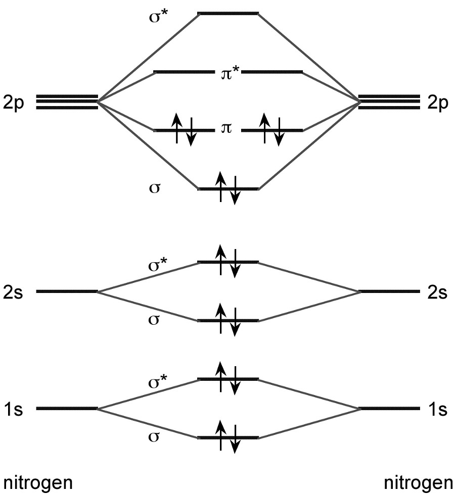
Note that this diagram does not take spin-orbit into account, but we shall consider this interaction later on. Let us first consider the possible final states. One electron leaves from one of four spin-orbitals and enters one of six spin-orbitals. This gives 24 determinants which translates into the following states:
| Configuration | States |
|---|---|
| \(1s\sigma_g^{-1}2p\pi_g\) | \(^{1,3}\Pi_g\) |
| \(1s\sigma_g^{-1}2p\sigma_u\) | \(^{1,3}\Sigma_u\) |
| \(1s\sigma_u^{-1}2p\pi_g\) | \(^{1,3}\Pi_u\) |
| \(1s\sigma_u^{-1}2p\sigma_u\) | \(^{1,3}\Sigma_g\) |
Spin-orbit free calculation
Preparing the input files
We employ the following molecular input file N2.mol
DIRAC
N2
cc-pVTZ basis
C   1              A
        7.    2
N1         0.0        0.0       0.00000
N2         0.0        0.0       1.09800
LARGE BASIS cc-pVTZ
FINISH
Here we do not provide any symmetry information, meaning that we ask DIRAC to detect it. DIRAC will find that the full group is \(D_{\infty h}\). With spin-orbit coupling DIRAC will then activate linear supersymmetry, but in the spin-orbit free case it will simply use the highest Abelian single point group, that is \(D_{2h}\). For the final states DIRAC will employ the total symmetry, that is the combined spin and spatial symmetry. Here we shall keep in mind that the singlet spin function is totally symmetric (\(A_g\)), whereas the triplet spin functions transform as rotations. We know the triplet functions as:
but for our purposes it will be more convenient to form the combinations:
which transform as rotations \(R_x\left(B_{3g}\right)\) , \(R_y\left(B_{2g}\right)\) and \(R_z\left(B_{1g}\right)\) , respectively.
We can now set up the following correlation of states:
| State | Spin | Spatial | Spin \(\otimes\) Spatial |
|---|---|---|---|
| \(^1\Sigma_g\) | \(A_g\) | \(A_g\) | \(A_g\) |
| \(^1\Sigma_u\) | \(A_g\) | \(B_{1u}\) | \(B_{1u}\) |
| \(^1\Pi_{x,y;g}\) | \(A_g\) | \(B_{3g}, B_{2g}\) | \(B_{3g}, B_{2g}\) |
| \(^1\Pi_{x,y;u}\) | \(A_g\) | \(B_{3u}, B_{2u}\) | \(B_{3u}, B_{2u}\) |
| \(^3\Sigma_g\) | \(B_{3g}, B_{2g}, B_{1g}\) | \(A_g\) | \(B_{3g}, B_{2g}, B_{1g}\) |
| \(^3\Sigma_u\) | \(B_{3g}, B_{2g}, B_{1g}\) | \(B_{1u}\) | \(B_{2u}, B_{3u}, A_{u}\) |
| \(^3\Pi_{x,y;g}\) | \(B_{3g}, B_{2g}, B_{1g}\) | \(B_{3g}, B_{2g}\) | \(\left(A_g, B_{1g}, B_{2g}\right), \left(B_{1g}, A_g, B_{3g}\right)\) |
| \(^3\Pi_{x,y;u}\) | \(B_{3g}, B_{2g}, B_{1g}\) | \(B_{3u}, B_{2u}\) | \(\left(A_u, B_{1u}, B_{2u}\right), \left(B_{1u}, A_u, B_{3u}\right)\) |
Counting total symmetries we find the 24 microstates are evenly distributed amongst the eight irreps of \(D_{2h}\):
| Irrep | Core-ionized state | |
|---|---|---|
| \(A_g\) | \(^1\Sigma_g, ^{3(x)}\Pi_{x;g}, ^{3(y)}\Pi_{y;g}\) | \(x^2, y^2, z^2\) |
| \(B_{3u}\) | \(^{1}\Pi_{x;u}, ^{3(y)}\Sigma_u, ^{3(z)}\Pi_{y;u}\) | \(x\) |
| \(B_{2u}\) | \(^{1}\Pi_{y;u}, ^{3(x)}\Sigma_u, ^{3(z)}\Pi_{x;u}\) | \(y\) |
| \(B_{1g}\) | \(^{3(z)}\Sigma_g, ^{3(y)}\Pi_{x;g}, ^{3(x)}\Pi_{y;g}\) | \(xy\) |
| \(B_{1u}\) | \(^1\Sigma_u, ^{3(y)}\Pi_{x;u}, ^{3(x)}\Pi_{y;u}\) | \(z\) |
| \(B_{2g}\) | \(^{1}\Pi_{y;g}, ^{3(y)}\Sigma_g, ^{3(z)}\Pi_{x;g}\) | \(xz\) |
| \(B_{3g}\) | \(^{1}\Pi_{x;g}, ^{3(x)}\Sigma_g, ^{3(z)}\Pi_{y;g}\) | \(yz\) |
| \(A_{u}\) | \(^{3(z)}\Sigma_u, ^{3(x)}\Pi_{x;u}, ^{3(y)}\Pi_{y;u}\) | \(xyz\) |
From these considerations we now set up the following menu file for our calculation
**DIRAC
.WAVE FUNCTION
.ANALYZE
.PROPERTIES
**INTEGRALS
*READIN
.UNCONTRACT
**HAMILTONIAN
.SPINFREE
.DFT
PBE0
**WAVE FUNCTION
.SCF
*SCF
.CLOSED SHELL
6 8
**ANALYZE
.MULPOP
*MULPOP
.VECPOP
1..5
1..5
**PROPERTIES
.PRINT
1
*EXCITATION ENERGIES
.OCCUP
1
1
.EXCITATIONS  !Ag
1 3
.EXCITATIONS  !B3u
2 3
.EXCITATIONS  !B2u
3 3
.EXCITATIONS  !B1g
4 3
.EXCITATIONS  !B1u
5 3
.EXCITATIONS  !B2g
6 3
.EXCITATIONS  !B3g
7 3
.EXCITATIONS  !Au
8 3
.INTENS
0
.ANALYZE
.SKIPEP
*END OF INPUT
In the *SCF section we give the electron occupation of \(N_2\): 6 and 8 electrons in gerade and ungerade orbitals, respectively. We also ask for a Mulliken population analysis (.MULPOP) for the occupied orbitals and the orbitals involved in the core excitation.
Let us now look at how we set up the calculation of excitation energies under *EXCITATION ENERGIES. We have seen that there are three excitations per boson irrep. Note that the numbering of irreps follow what you for instance find in the \(D_{2h}\) direct product table in the output:
|   | Ag   B3u  B2u  B1g  B1u  B2g  B3g  Au
-----+----------------------------------------
Ag  | Ag   B3u  B2u  B1g  B1u  B2g  B3g  Au
B3u | B3u  Ag   B1g  B2u  B2g  B1u  Au   B3g
B2u | B2u  B1g  Ag   B3u  B3g  Au   B1u  B2g
B1g | B1g  B2u  B3u  Ag   Au   B3g  B2g  B1u
B1u | B1u  B2g  B3g  Au   Ag   B3u  B2u  B1g
B2g | B2g  B1u  Au   B3g  B3u  Ag   B1g  B2u
B3g | B3g  Au   B1u  B2g  B2u  B1g  Ag   B3u
Au  | Au   B3g  B2g  B1u  B1g  B2u  B3u  Ag
Note also that we skip excitations in \(B_{2u}\) and \(B_{2g}\), since they are related by symmetry to the excitations of \(B_{3u}\) and \(B_{3g}\), respectively.
If nothing further is specified the excitation energies are calculated by a “bottoms-up” approach and so we will get valence excitations only, since the core-excitations are much higher in energy. We therefore restrict the excitations to the occupied \(1s\sigma_g\) and \(1s\sigma_u\) orbitals.
We furthermore ask for transition moments to be calculated with respect to the component of the dipole moment operator. These will be non-zero only for excitations in irreps \(B_{3u}, B_{2u}\) and \(B_{1u}\). Finally we ask for analysis of what orbitals contribute to the various excitations. For this the Mulliken population analysis may come in handy as reference.
Looking at the output
After running the calculation, let us now look at the output. The following excitation energies were calculated
 Level   Rel eigenvalue     Abs eigenvalue      Total Energy    Degeneracy

    0     0.0000000000      0.000000000000     -109.506175626874 (   1 * )
    1    14.2873900530     14.287390053039      -95.218785573835 (   2 * )
    2    14.2873901429     14.287390142869      -95.218785484005 (   2 * )
    3    14.2874014745     14.287401474486      -95.218774152388 (   2 * )
    4    14.2892617095     14.289261709468      -95.216913917405 (   2 * )
    5    14.2892617988     14.289261798798      -95.216913828075 (   2 * )
    6    14.2892731363     14.289273136296      -95.216902490578 (   2 * )
    7    14.3291612539     14.329161253885      -95.177014372989 (   2 * )
    8    14.3298947237     14.329894723671      -95.176280903203 (   2 * )
    9    14.6936222414     14.693622241426      -94.812553385448 (   1 * )
   10    14.6936223755     14.693622375464      -94.812553251410 (   2 * )
   11    14.6951870758     14.695187075770      -94.810988551103 (   1 * )
   12    14.6951872031     14.695187203115      -94.810988423758 (   2 * )
   13    14.7188072608     14.718807260844      -94.787368366029 (   1 * )
   14    14.7206158042     14.720615804223      -94.785559822650 (   1 * )
DIRAC assumes that excitation energies that are within \(10^{-9}\ E_h\) of each other come from the same degenerate state. This threshold is somewhat arbitrary and we shall see that DIRAc is not always correct.
There is sufficient symmetry in the calculation (symmetry distinct rotation) to allow DIRAC to pinpoint the symmetry of the core-ionized state and we therefore find the following distribution
 Level  eigenvalue (eV)  Eigenvalue (cm-1)  1Ag |1B3u|1B2u|1B1g|1B1u|1B2g|1B3g|1Au |

    0        0.000000000          0.000000     1|   0|   0|   0|   0|   0|   0|   0|
    1      388.779649059    3135719.663853     0|   0|   0|   0|   0|   0|   0|   0|
    2      388.779651503    3135719.683569     0|   0|   0|   0|   0|   0|   0|   0|
    3      388.779959852    3135722.170571     0|   0|   0|   0|   0|   0|   0|   0|
    4      388.830579420    3136130.444958     0|   0|   0|   0|   0|   0|   0|   0|
    5      388.830581850    3136130.464564     0|   0|   0|   0|   0|   0|   0|   0|
    6      388.830890359    3136132.952857     0|   0|   0|   0|   0|   0|   0|   0|
    7      389.916301222    3144887.382757     0|   1|   1|   0|   0|   0|   0|   0|
    8      389.936259949    3145048.360768     0|   0|   0|   0|   0|   1|   1|   0|
    9      399.833788902    3224877.323614     0|   0|   0|   0|   0|   0|   0|   0|
   10      399.833792549    3224877.353032     0|   0|   0|   0|   0|   0|   0|   0|
   11      399.876370209    3225220.765055     0|   0|   0|   0|   0|   0|   0|   0|
   12      399.876373674    3225220.793004     0|   0|   0|   0|   0|   0|   0|   0|
   13      400.519108122    3230404.796465     1|   0|   0|   0|   0|   0|   0|   0|
   14      400.568321089    3230801.725856     0|   0|   0|   0|   1|   0|   0|   0|


 Relative real eigenvalues in other units;
 Symmetry Classification in the Abelian subgroup

 Level  eigenvalue (eV)  Eigenvalue (cm-1)  3Ag |3B3u|3B2u|3B1g|3B1u|3B2g|3B3g|3Au |

    0        0.000000000          0.000000     0|   0|   0|   0|   0|   0|   0|   0|
    1      388.779649059    3135719.663853     0|   1|   1|   0|   0|   0|   0|   0|
    2      388.779651503    3135719.683569     0|   1|   1|   0|   0|   0|   0|   0|
    3      388.779959852    3135722.170571     0|   1|   1|   0|   0|   0|   0|   0|
    4      388.830579420    3136130.444958     0|   0|   0|   0|   0|   1|   1|   0|
    5      388.830581850    3136130.464564     0|   0|   0|   0|   0|   1|   1|   0|
    6      388.830890359    3136132.952857     0|   0|   0|   0|   0|   1|   1|   0|
    7      389.916301222    3144887.382757     0|   0|   0|   0|   0|   0|   0|   0|
    8      389.936259949    3145048.360768     0|   0|   0|   0|   0|   0|   0|   0|
    9      399.833788902    3224877.323614     1|   0|   0|   0|   0|   0|   0|   0|
   10      399.833792549    3224877.353032     2|   0|   0|   0|   0|   0|   0|   0|
   11      399.876370209    3225220.765055     0|   0|   0|   0|   1|   0|   0|   0|
   12      399.876373674    3225220.793004     0|   0|   0|   0|   2|   0|   0|   0|
   13      400.519108122    3230404.796465     0|   0|   0|   0|   0|   0|   0|   0|
   14      400.568321089    3230801.725856     0|   0|   0|   0|   0|   0|   0|   0|
The first and second block refers to singlet and triplet states, respectively. Based on the discussion in the preceeding section we see that levels 1, 2 and 3 all come from a \(^3\Pi_u\) which in \(D_{2h}\) splits into \(^3B_{2u}\) and \(^3B_{3u}\). After careful inspection we can set up the following table
| Level | eigenvalue (eV) | |
|---|---|---|
| 0 | 0.000 | \(^1\Sigma_g\) |
| 1,2,3 | 388.780 | \(^3\Pi_u\) |
| 4,5,6 | 388.831 | \(^3\Pi_g\) |
| 7 | 389.916 | \(^1\Pi_u\) |
| 8 | 389.936 | \(^1\Pi_g\) |
| 9,10 | 399.834 | \(^3\Sigma_g\) |
| 11,12 | 399.876 | \(^3\Sigma_u\) |
| 13 | 400.519 | \(^1\Sigma_g\) |
| 14 | 400.568 | \(^1\Sigma_u\) |
Looking further down in the output we find dominant inactive and virtual orbitals. Restricting attention to \(B_{3u}\) total symmetry we find that the first excited state \(^3\Pi_u\), at 388.78 eV, is dominated by the excitation 1(i:E1u) —> 4(v:E1g), which, as can be inferred from the Mulliken population analysis, corresponds to \(1s\sigma_u \rightarrow 2p\pi_{y;g}\). The second excited state \(^1\Pi_u\), at 389.91 eV, corresponds to 1(i:E1u) —> 5(v:E1g) (\(1s\sigma_u \rightarrow 2p\pi_{x;g}\)), whereas the third excited state \(^3\Sigma_u\), at 399.88 eV, is dominated by 1(i:E1g) —> 5(v:E1u) (\(1s\sigma_g \rightarrow 2p\sigma_u\)).
Within the electric dipole approximation only singlet states get oscillator strengths. In the output we find
* ISOTROPIC DL-DL OSCILLATOR STRENGTHS (f)
==========================================
DL = dipole length
Rate = Dipole radiation rate (s-1)
Lifetime = corresponding radiation lifetime (s)

Level     Frequency     f             Rate           Lifetime
------------------------------------------------------------------------
   14    14.3291612539  0.11150564    0.73561E+12    0.13594E-11   1B3u
   15    14.3291612539  0.11150564    0.73561E+12    0.13594E-11   1B2u
   25    14.7206158042  0.00007988    0.55615E+09    0.17981E-08   1B1u
------------------------------------------------------------------------
Sum of oscillator strenghts:      0.22309
showing intensity to the \(^1\Pi_u\) and \(^1\Sigma_u\) states.
Including spin-orbit
Spin-orbit is included by simply commenting out the keyword .SPINFREE in the input above:
**HAMILTONIAN
!.SPINFREE
This leads to the following states:
 Level   Rel eigenvalue     Abs eigenvalue      Total Energy    Degeneracy

    0     0.0000000000      0.000000000000     -109.506177757989 (   1 * )
    1    14.2870674366     14.287067436576      -95.219110321412 (   1 * )
    2    14.2870902909     14.287090290867      -95.219087467121 (   1 * )
    3    14.2873870516     14.287387051622      -95.218790706367 (   2 * )
    4    14.2877107670     14.287710767041      -95.218466990947 (   2 * )
    5    14.2889390867     14.288939086714      -95.217238671275 (   1 * )
    6    14.2889619501     14.288961950065      -95.217215807924 (   1 * )
    7    14.2892586419     14.289258641924      -95.216919116065 (   2 * )
    8    14.2895824310     14.289582431019      -95.216595326970 (   2 * )
    9    14.3291623896     14.329162389555      -95.177015368434 (   2 * )
   10    14.3298959259     14.329895925905      -95.176281832084 (   2 * )
   11    14.6936210547     14.693621054697      -94.812556703291 (   1 * )
   12    14.6936211889     14.693621188921      -94.812556569068 (   2 * )
   13    14.6951858891     14.695185889130      -94.810991868859 (   1 * )
   14    14.6951860166     14.695186016639      -94.810991741349 (   2 * )
   15    14.7188060692     14.718806069152      -94.787371688837 (   1 * )
   16    14.7206146122     14.720614612164      -94.785563145825 (   1 * )
with the following distribution on linear symmetries:
 Level  eigenvalue (eV)  Eigenvalue (cm-1)   0g+| 0g-| 1g | 2g | 0u+| 0u-| 1u | 2u |

    0        0.000000000          0.000000     1|   0|   0|   0|   0|   0|   0|   0|
    1      388.770870219    3135648.857724     0|   0|   0|   0|   1|   0|   0|   0|
    2      388.771492115    3135653.873661     0|   0|   0|   0|   0|   1|   0|   0|
    3      388.779567386    3135719.005118     0|   0|   0|   0|   0|   0|   2|   0|
    4      388.788376130    3135790.052441     0|   0|   0|   0|   0|   0|   0|   2|
    5      388.821800408    3136059.637448     1|   0|   0|   0|   0|   0|   0|   0|
    6      388.822422551    3136064.655374     0|   1|   0|   0|   0|   0|   0|   0|
    7      388.830495947    3136129.771710     0|   0|   2|   0|   0|   0|   0|   0|
    8      388.839306697    3136200.835202     0|   0|   0|   2|   0|   0|   0|   0|
    9      389.916332125    3144887.632008     0|   0|   0|   0|   0|   0|   2|   0|
   10      389.936292664    3145048.624628     0|   0|   2|   0|   0|   0|   0|   0|
   11      399.833756609    3224877.063157     0|   1|   0|   0|   0|   0|   0|   0|
   12      399.833760262    3224877.092616     0|   0|   2|   0|   0|   0|   0|   0|
   13      399.876337919    3225220.504617     0|   0|   0|   0|   0|   1|   0|   0|
   14      399.876341389    3225220.532602     0|   0|   0|   0|   0|   0|   2|   0|
   15      400.519075694    3230404.534918     1|   0|   0|   0|   0|   0|   0|   0|
   16      400.568288652    3230801.464229     0|   0|   0|   0|   1|   0|   0|   0|
Comparing with the preceeding section we see the following spin-orbit decomposition of the :math:Lambda-S` states:
| Level | eigenvalue (eV) | ||
|---|---|---|---|
| 0 | 0.000 | \(^1\Sigma^+_g\) | \(0_g^+\) (0.000) |
| 1,2,3 | 388.780 | \(^3\Pi_u\) | \(0^+_u\) (388.771), \(0^-_u\) (388.771), \(1_u\) (388.780), \(2_u\) (388.788) |
| 4,5,6 | 388.831 | \(^3\Pi_g\) | \(0^+_g\) (388.821), \(0^-_g\) (388.822), \(1_g\) (388.830), \(2_g\) (388.839) |
| 7 | 389.916 | \(^1\Pi_u\) | \(1_u\) (389.916) |
| 8 | 389.936 | \(^1\Pi_g\) | \(1_g\) (389.936) |
| 9,10 | 399.834 | \(^3\Sigma^+_g\) | \(0^-_g\) (399.834), \(1_g\) (399.834) |
| 11,12 | 399.876 | \(^3\Sigma^+_u\) | \(0^-_u\) (399.876), \(1_u\) (399.876) |
| 13 | 400.519 | \(^1\Sigma^+_g\) | \(0^+_g\) (400.519) |
| 14 | 400.568 | \(^1\Sigma^+_u\) | \(0^+_u\) (400.568) |
Note that the energies are given relative to the lowest level, that is, the ground state and that it is somewhat stabilized by spin-orbit coupling.
The effect of spin-orbit coupling shows up in the oscillator strengths:
Level     Frequency     f             Rate           Lifetime
------------------------------------------------------------------------
    2    14.2870674366  0.00000008    0.52188E+06    0.19161E-05    0u+
    4    14.2873870516  0.00000617    0.40461E+08    0.24715E-07    1u
    5    14.2873870516  0.00000617    0.40461E+08    0.24715E-07    1u
   14    14.3291623896  0.11149933    0.73557E+12    0.13595E-11    1u
   15    14.3291623896  0.11149933    0.73557E+12    0.13595E-11    1u
   25    14.7206146122  0.00007988    0.55616E+09    0.17981E-08    0u+
------------------------------------------------------------------------
Sum of oscillator strenghts:      0.22309
What we see is the \(0_u^+\) and \(1_u\) components of the \(^3\Pi_u\) state stealing intensity from the singlet states. This change is not very spectacular since the nitrogen molecule is composed of light atoms for which relativistic effects are not very strong. We can mimic a more strongly relativistic system by reducing the speed of light to e.g. 20 a.u.:
**GENERAL
.CVALUE
20.0D0
We now see
Level     Frequency     f             Rate           Lifetime
------------------------------------------------------------------------
    2    14.7249228123  0.00019318    0.13458E+10    0.74305E-09    0u+
    6    14.7354731379  0.01012800    0.70658E+11    0.14153E-10    1u
    7    14.7354731379  0.01012800    0.70658E+11    0.14153E-10    1u
   14    14.7841864012  0.09369466    0.65799E+12    0.15198E-11    1u
   15    14.7841864012  0.09369466    0.65799E+12    0.15198E-11    1u
   22    15.1211545881  0.00000251    0.18439E+08    0.54232E-07    1u
   23    15.1211545881  0.00000251    0.18439E+08    0.54232E-07    1u
   25    15.1494320202  0.00006483    0.47805E+09    0.20918E-08    0u+
------------------------------------------------------------------------
Sum of oscillator strenghts:      0.20791