Magnetizability density

In this tutorial we will plot the CGO magnetizability density of the water molecule. We will do this in two steps: first we will run the SCF and response calculation and save the CHECKPOINT.h5, PAMXVC, and RESPONSE.h5 files, then we will restart from these and calculate the magnetizability density on a grid of points and write this into a cube file which can be opened by your favorite molecular visualization program (the author of this tutorial likes Avogadro).

Tip: it might be helpful to check the analysis of other magnetic response densities in a Jupyter notebook in ../../../../demo_notebooks/visual_overview.ipynb.

Getting the wave function and the response vectors

Let us use the following molecule input (h2o.mol):

DIRAC


C   2    0
        1.    2
H    -1.4523499293         .0000000000         .8996235720
H     1.4523499293         .0000000000         .8996235720
LARGE BASIS cc-pVDZ
        8.    1
O      .0000000000        0.0000000000        -.2249058930
LARGE BASIS cc-pVDZ
FINISH

Together with a simple job input (magnetizability.inp):

**DIRAC
.WAVE FUNCTION
.PROPERTIES
**HAMILTONIAN
.DFT
 B3LYP
**WAVE FUNCTION
.SCF
**PROPERTIES
.MAGNETIZABILITY
*LINEAR RESPONSE
.RSPEXP
*END OF INPUT

We can get the wave function with the following run script:

pam --inp=magnetizability.inp --mol=h2o.mol --get="CHECKPOINT.h5 PAMXVC RESPONSE.h5"

After running the script you should see the files CHECKPOINT.h5 and PAMXVC in your submit directory.

And here is the magnetizability tensor:

            Total magnetizability tensor (au)
            ---------------------------------

                     Bx                  By                  Bz


Bx        -1.804460514289     -0.000000000000     -0.000000000001
By        -0.000000000000     -1.617444735515      0.000000000000
Bz        -0.000000000001     -0.000000000000     -1.709814652525

Plotting the magnetizability density

We will use the following run script to generate the cube file:

pam --inp=density.inp --mol=h2o.mol --put="CHECKPOINT.h5 PAMXVC" --get=plot.3d.cube

Together with the following job input (density.inp):

**DIRAC
#.WAVE FUNCTION
**HAMILTONIAN
.DFT
 B3LYP
**WAVE FUNCTION
.SCF
**VISUAL
.GRIDS
1
id=1 input=create typ=1 npoints=[80,80,80] margin=4.0
.GRIDFUNCTIONS
6
name=bdip id_grid=1 purpose=visualization export=txt rspvec_file=RESPONSE.h5 rspvec_id=1 file_out=bdip_Bz_rspvec1.txt
name=bdip id_grid=1 purpose=visualization export=txt rspvec_file=RESPONSE.h5 rspvec_id=2 file_out=bdip_Bz_rspvec2.txt
name=bdip id_grid=1 purpose=visualization export=txt rspvec_file=RESPONSE.h5 rspvec_id=3 file_out=bdip_Bz_rspvec3.txt
name=bdip id_grid=1 purpose=visualization export=txt rspvec_file=RESPONSE.h5 rspvec_id=4 file_out=bdip_Bz_rspvec4.txt
name=bdip id_grid=1 purpose=visualization export=txt rspvec_file=RESPONSE.h5 rspvec_id=5 file_out=bdip_Bz_rspvec5.txt
name=bdip id_grid=1 purpose=visualization export=txt rspvec_file=RESPONSE.h5 rspvec_id=6 file_out=bdip_Bz_rspvec6.txt
*END OF INPUT

Finally you can open cube files with your favorite program and visualize the density. You can sum up all contributions to the total density or plot specific components or paramagnetic and diamagnetic contributions separately.

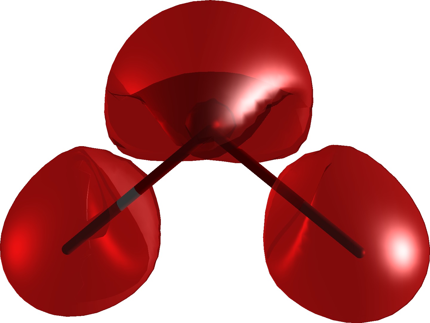
And this is how the total magnetizability density of water looks (isosurface 0.04 a.u.):