xamfX2C: Two-electon picture change corrections for the X2C Hamiltonian
This tutorial demonstrates the usage and usefulness of the (extended) atomic mean-field two-electron picture-change corrections for the X2C Hamiltonian.
Short theory
The goal is to reproduce total energy and orbital energies of a 4-component SCF calculation as accurate as possible at the 2-component level. Restricting ourselves first to Hartree-Fock theory, this would require using the correctly transformed set of one- and two-electron integrals
where \(X,Y,U,V\in L,S\) and \(U\) is the picture-change transformation matrix that correctly block-diagonalizes the converged 4-component Fock matrix \(F^{4c}\).
For more information on the actual details of the theory and implementation see Ref. [Knecht2022].
A gold complex: \([{\rm Au(Cl)}_4]^-\)
We first consider a Au(III)-complex, tetrachloroaurate.
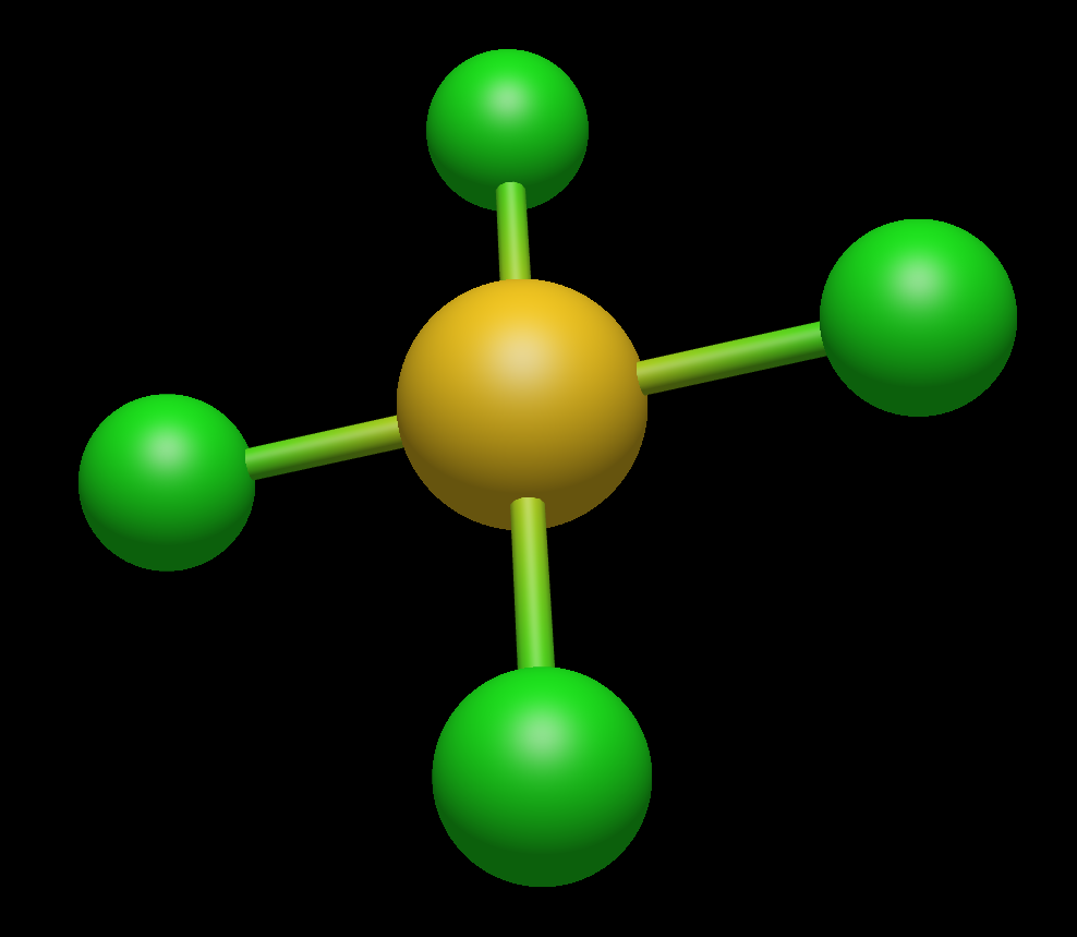
Using the structure given in [Hargittai_JACS2001] (Table I: column MP2/aug-cc-pVTZ), we prepare the following xyz-file
5
MP2/aug-TZ optimized from JACS, 123, 1449-1458 (2001).
Au                 0.00000000    0.00000000    0.00000000
Cl                 0.00000000    2.2930000000  0.00000000
Cl                 0.00000000   -2.2930000000  0.00000000
Cl                 2.2930000000  0.00000000    0.00000000
Cl                -2.2930000000  0.00000000    0.00000000
Warning
Notice that by default, for the total energy, DIRAC uses the simple Coulombic correction introduced by [Visscher1997a], where the calculation of the expensive (SS|SS)-class of integrals is avoided by introducing an energy correction in terms of the repulsion of small component atomic charges. The amfX2C (and eamfX2C) model tries to reproduce 4-component total and orbital energies for a general molecule based on information extracted from atomic 4-component relativistic calculations. Since these are relatively cheap, we strongly recommend including the (SS|SS)-class of integrals in these atomic calculations.
Reference calculation
For reference, we therefore carry out a 4-component relativistic Hartree-Fock calculation with (SS|SS)-class of integrals included. We use the dyall.v2z basis set. Our menu file therefore looks like:
**DIRAC
.TITLE
AuCl4-
.WAVE F
**HAMILTONIAN
.DOSSSS
**WAVE FUNCTIONS
.SCF
*SCF
.CLOSED SHELL
 74 74
**MOLECULE
*BASIS
.DEFAULT
 dyall.v2z
*END OF
and can be run using:
pam --inp=4c --mol=AuCl4.xyz
In the output we then find:
                               TOTAL ENERGY
                               ------------

Charge of molecule : -1

Electronic energy                        :    -22374.645394444109

Other contributions to the total energy
Nuclear repulsion energy                 :      1495.084959925113

Sum of all contributions to the energy
Total energy                             :    -20879.560434518997
as well as occupied orbital energies:
* Fermion symmetry E1g
   * Closed shell, f = 1.0000
    -2986.172433056  ( 2)       -532.228239826  ( 2)       -128.126822999  ( 2)       -105.062162391  ( 4)        -85.994500068  ( 2)
      -85.992245877  ( 2)        -82.776253554  ( 2)        -82.773843683  ( 2)        -82.772814925  ( 2)        -29.176725071  ( 2)
      -13.906134621  ( 2)        -13.898588891  ( 2)        -13.210720978  ( 2)        -13.203947809  ( 2)        -13.203621787  ( 2)
      -10.449079002  ( 4)         -7.890617059  ( 4)         -7.827509378  ( 4)         -7.825980274  ( 4)         -4.715673601  ( 2)
       -0.929177412  ( 2)         -0.904022207  ( 2)         -0.533120234  ( 2)         -0.505514832  ( 2)         -0.457699080  ( 2)
       -0.454463761  ( 2)         -0.429307565  ( 2)         -0.354242187  ( 2)         -0.290147741  ( 2)         -0.270966594  ( 2)
       -0.265726870  ( 2)         -0.252693231  ( 2)

 * Fermion symmetry E1u
   * Closed shell, f = 1.0000
     -509.312470287  ( 2)       -441.741820331  ( 2)       -441.741607132  ( 2)       -117.884404188  ( 2)       -105.062163078  ( 4)
     -102.771317291  ( 2)       -102.767075769  ( 2)        -24.775448231  ( 2)        -21.109216293  ( 2)        -21.099913774  ( 2)
      -10.449103312  ( 4)         -7.890617462  ( 4)         -7.827509914  ( 4)         -7.825980151  ( 4)         -3.911755156  ( 2)
       -3.901812050  ( 2)         -3.898146885  ( 2)         -3.763318698  ( 2)         -3.756380303  ( 2)         -3.751940592  ( 2)
       -3.750335458  ( 2)         -3.216879082  ( 2)         -2.570010773  ( 2)         -2.569726879  ( 2)         -0.901102780  ( 2)
       -0.898562174  ( 2)         -0.333968015  ( 2)         -0.325038247  ( 2)         -0.316265455  ( 2)         -0.284482135  ( 2)
       -0.270870860  ( 2)         -0.268370374  ( 2)
amfX2C calculation
Initial atomic calculations
As preparation to a amfX2C (or eamfX2C) calculation we need to carry out 4-component relativistic atomic calculations. For gold we use the menu file
**DIRAC
.WAVE FUNCTION
.ANALYZE
**HAMILTONIAN
.X2Cmmf
.DOSSSS
*X-AMFI
.amf
**WAVE FUNCTION
.SCF
*SCF
.CLOSED SHELL
 40 38
.OPEN SHELL
1
1/2,0
**ANALYZE
.MULPOP
**MOLECULE
*BASIS
.DEFAULT
 dyall.v2z
**END OF
as well as the xyz-file
1

Au 0.0 0.0 0.0
Notice that we have specified the keyword .X2Cmmf. This means that DIRAC will run a 4-component relativistic Hartree-Fock calculation and then transform the converged Fock matrix to 2-component form. As recommended, we have included the .DOSSSS keyword to include the (SS|SS)-class of integrals. We have also specified the keyword .AMF such that the amfX2C corrections are prepared and written to file amfPCEC.h5. We run the gold calculation using:
pam --inp=Au.inp --mol=Au.xyz --get "amfPCEC.h5=amfPCEC.079.h5"
In similar manner, for chlorine we use the menu file
**DIRAC
.WAVE FUNCTION
.ANALYZE
**HAMILTONIAN
.X2Cmmf
.DOSSSS
*X-AMFI
.amf
**WAVE FUNCTION
.SCF
*SCF
.CLOSED SHELL
6 6
.OPEN SHELL
1
5/0,6
**ANALYZE
.MULPOP
**MOLECULE
*BASIS
.DEFAULT
 dyall.v2z
**END OF
as well as the xyz-file
1

Cl 0.000 0.000 0.000
and run the atomic calculation as:
pam --inp=Cl.inp --mol=Cl.xyz --get "amfPCEC.h5=amfPCEC.017.h5"
As a final preparatory step we have to merge the generated correction files:
$BUILD_DIR/merge_amf.py amfPCEC.079.h5 amfPCEC.017.h5
Molecular calculation
We are now set for the molecular amfX2C calculation. We use the menu file
**DIRAC
.TITLE
AuCl4-
.WAVE F
**HAMILTONIAN
.X2C
*X-AMFI
.amf
**WAVE FUNCTIONS
.SCF
*SCF
.CLOSED SHELL
 74 74
**MOLECULE
*BASIS
.DEFAULT
 dyall.v2z
*END OF
and run the calculation using:
pam --inp=amfX2C.inp --mol=AuCl4.xyz --put="amfPCEC.h5"
In the output we now find:
                                TOTAL ENERGY
                                ------------

Charge of molecule : -1

Electronic energy                        :    -22374.646183410361
... with amf contributions to 2e-energy  :        -6.730906332501

Other contributions to the total energy
Nuclear repulsion energy                 :      1495.084959925113

Sum of all contributions to the energy
Total energy                             :    -20879.561223485249
as well as orbital energies:
* Fermion symmetry E1g
   * Closed shell, f = 1.0000
    -2986.172409644  ( 2)       -532.228297520  ( 2)       -128.126807822  ( 2)       -105.062171345  ( 4)        -85.994478858  ( 2)
      -85.992230143  ( 2)        -82.776268135  ( 2)        -82.773836896  ( 2)        -82.772797520  ( 2)        -29.176705603  ( 2)
      -13.906104864  ( 2)        -13.898568611  ( 2)        -13.210714521  ( 2)        -13.203931944  ( 2)        -13.203597745  ( 2)
      -10.449084871  ( 4)         -7.890622640  ( 4)         -7.827525601  ( 4)         -7.825972582  ( 4)         -4.715657228  ( 2)
       -0.929176110  ( 2)         -0.904021904  ( 2)         -0.533079011  ( 2)         -0.505500573  ( 2)         -0.457674033  ( 2)
       -0.454442417  ( 2)         -0.429318493  ( 2)         -0.354227188  ( 2)         -0.290151069  ( 2)         -0.270967632  ( 2)
       -0.265733913  ( 2)         -0.252693395  ( 2)
 * Fermion symmetry E1u
    * Closed shell, f = 1.0000
     -509.312585352  ( 2)       -441.741860248  ( 2)       -441.741615553  ( 2)       -117.884391655  ( 2)       -105.062172090  ( 4)
     -102.771297597  ( 2)       -102.767054981  ( 2)        -24.775425636  ( 2)        -21.109198160  ( 2)        -21.099888900  ( 2)
      -10.449109460  ( 4)         -7.890623044  ( 4)         -7.827526119  ( 4)         -7.825972449  ( 4)         -3.911723029  ( 2)
       -3.901789268  ( 2)         -3.898128341  ( 2)         -3.763312842  ( 2)         -3.756362106  ( 2)         -3.751916324  ( 2)
       -3.750305598  ( 2)         -3.216839463  ( 2)         -2.570027444  ( 2)         -2.569697960  ( 2)         -0.901108027  ( 2)
       -0.898559198  ( 2)         -0.333966781  ( 2)         -0.325040872  ( 2)         -0.316260263  ( 2)         -0.284482236  ( 2)
       -0.270861088  ( 2)         -0.268373653  ( 2)
Comparison with the 4-component reference, shows that the total energy has an error of -0.7 mH, whereas the mean absolute error in the orbital energies is 5.69 \(\mu\mbox{H}\). If we do not use the (SS|SS)-integrals, that is, we remove the keyword .DOSSSS from the preparatory 4-component atomic calculations, as well as the 4-component molecular reference calculation, then the error in the total energy is still -0.7 mH, but the mean absolute error in the orbital energies increases to 51.1 \(\mu\mbox{H}\). It is also possible to go the other way: If we do add the Gaunt term using the keyword .GAUNT, then the error in total energy is -1.73 mH, and the mean absolute error in orbital energies is -3.79 \(\mu\mbox{H}\).
Core-ionization energies
A very nice feature of the amfX2C approach is that the two-electron picture-change corrections adapt to the computational setup. For instance, if we do a Kohn-Sham calculation instead of Hartree-Fock, the corrections are generated for our specific choice of functional as well as basis set. As an example, let us consider core-ionization energies, arising from gold \(2p_{1/2}\ (L_2)\) and \(2p_{3/2}\ L_3\) for our gold complex, calculated using the PBE0 functional. The preparatory atomic calculations as well as the amfX2C calculation proceeds as before, except that we have inserted:
.DFT
PBE0
in the **HAMILTONIAN section. In the amfX2C calculation, we have also asked for a Mulliken population analysis and find for fermion ircip \(E_{1u}\):
* Electronic eigenvalue no.   1: -503.04886526180       (Occupation : f = 1.0000)
============================================================================================

* Gross populations greater than 0.01000

Gross     Total   |    L B3uAu px     L B2uAu py     L B1uAu pz
--------------------------------------------------------------------
 alpha    0.3333  |      0.0000         0.0000         0.3333
 beta     0.6667  |      0.3333         0.3333         0.0000

* Electronic eigenvalue no.   2: -435.57080277128       (Occupation : f = 1.0000)
============================================================================================

* Gross populations greater than 0.01000

Gross     Total   |    L B3uAu px     L B2uAu py
-----------------------------------------------------
 alpha    0.0000  |      0.0000         0.0000
 beta     1.0000  |      0.5000         0.5000

* Electronic eigenvalue no.   3: -435.56940890418       (Occupation : f = 1.0000)
============================================================================================

* Gross populations greater than 0.01000

Gross     Total   |    L B3uAu px     L B2uAu py     L B1uAu pz
--------------------------------------------------------------------
 alpha    0.6667  |      0.0000         0.0000         0.6667
 beta     0.3333  |      0.1667         0.1667         0.0000
Let us now calculate binding energy of these orbitals by \(\Delta SCF\). For the \(L_2\)-edge we prepare the menu file L2_amfX2C.inp
**DIRAC
.TITLE
AuCl4-
.WAVE F
.ANALYZE
**HAMILTONIAN
.X2C
.DFT
PBE0
*X-AMFI
.amf
**WAVE FUNCTIONS
.SCF
.REORDER
1..37
2..37,1
*SCF
.CLOSED SHELL
 74 72
.OPEN SHELL
1
1.0/0,2
.OVLSEL
.NODYNSEL
**ANALYZE
.MULPOP
**MOLECULE
*BASIS
.DEFAULT
 dyall.v2z
*END OF
This is an open-shell system, at the Kohn-Sham level calculated using fractional occupation. In DIRAC, positive-energy solutions are sorted first with respect to orbital class (closed, open, virtual), then with respect to orbital energies. We therefore use the keyword .REORDER MO to bring the now singly occupied gold \(2p_{1/2}\) orbital just after the occupied orbitals of ungerade symmetry. We also use overlap selection to keep the orbital in that position during the SCF iteration. Specifially, we active overlap selection with the keyword .OVLSEL and in addition use .NODYNSEL so that overlap is always calculated with respect to the inital set of orbitals. We run the calculation using:
pam --inp=L2_amfX2C.inp --mol=AuCl4.xyz --put "amfX2C_AuCl4.h5=CHECKPOINT.h5 amfPCEC.h5" --noh5
Note that we added the –noh5 flag since we do not want to keep the associated checkpoint file. For each of the two \(2p_{3/2}\) we proceed in similar manner, simply modifying the reordering, using:
.REORDER
1..37
1,3..37,2
and:
.REORDER
1..37
1,2,4..37,3
Methane (\({\rm CH}_4\)) - The ultrarelativistic case
In the following example, we will calculate total energies and spinor energies of CH \(_4\) with several different Hamiltonians within the framework of DFT/PBE/dyall.v2z.
For convenience, in the Table below (see also Table IX in Ref. [Knecht2022]), we summarise the SCF total energy (E) and spinor energies (\(\epsilon\)) of the doubly degenerate occupied spinors for \({\rm CH}_4\) as obtained from DFT/PBE/v2z calculations within a four-component Dirac–Coulomb (\(^4{\rm DC}\)) as well as a two-component Hamiltonian framework, including the \({\rm (e)amfX2C}_{\rm DC}\) models. All energies are given in Hartree. The speed of light \(c\) was reduced by a factor 10.
\({\rm 1eX2C}_{\rm D}\) |
\({\rm AMFIX2C}_{\rm D}\) |
\({\rm amfX2C}_{\rm DC}\) |
\({\rm eamfX2C}_{\rm DC}\) |
\({}^{4}{\rm DC}\) |
|
|---|---|---|---|---|---|
E |
-42.14220 |
-42.14039 |
-42.26469 |
-42.25774 |
-42.25850 |
\(\epsilon_1\) |
-10.22206 |
-10.22401 |
-10.36154 |
-10.36028 |
-10.35794 |
\(\epsilon_2\) |
-0.65939 |
-0.65966 |
-0.66288 |
-0.66269 |
-0.66274 |
\(\epsilon_3\) |
-0.35705 |
-0.35288 |
-0.35649 |
-0.35291 |
-0.35290 |
\(\epsilon_{4-5}\) |
-0.33313 |
-0.33503 |
-0.33282 |
-0.33527 |
-0.33544 |
In order to make use of the (e)amf two-electron picture-change corrections, we will need to run atomic calculations for each element / nuclei type in the molecule. Hence, in the present case, we will run atomic calculations for C and H, respectively. The latter seems odd as H is by definition a one-electron system but as we will see, the MO coefficients will be needed for the \({\rm eamfX2C}_{\rm DC}\) model.
For a detailed discussion of the performance of the various picture-change correction models for the X2C Hamiltonian in comparison with the four-component reference data, we refer the interested user to Ref. [Knecht2022]. Let us highlight, though, that for the particular case of \({\rm eamfX2C}_{\rm DC}\) all picture-change correction terms for DFT (and likewise HF) are derived in molecular basis on the basis of molecular densities which are built from a superposition of atomic input densities. Consequently, in contrast to the simpler \({\rm amfX2C}_{\rm DC}\) model, the former comprises atomic contributions regardless of the actual atom type, that is, both “light” (one-electron) and “heavy” (many-electron) atoms contribute equally. Bearing the latter in mind, the total SCF energies as well as spinor energies compiled in the above Table confirm the unique numerical performance of the \({\rm eamfX2C}_{\rm DC}\) Hamiltonian model in comparison to the \({}^4{\rm DC}\) reference data.
Atomic calculations
Warning
Note that, besides scaling the speed of light by a factor of \(c\)/10, we also use a point nucleus as well as a different set of constants as default in our calculations. This was done for Ref. [Knecht2022] to match calculations with ReSpect. Since we would like to reproduce in this tutorial the results from Ref. [Knecht2022], we will keep those details. Needless to say, the \({\rm eamf}\) model works for finite nuclei just as for point nuclei.
H atom
For the atomic run of H, we use the following input (h.inp)
**DIRAC
.WAVE FUNCTION
**INTEGRAL
.NUCMOD
 1
*READIN
.UNCONTRACTED
**GENERAL
.CVALUE
13.703599907400d0
.CODATA
 CODATA10
**HAMILTONIAN
.X2Cmmf
.DOSSSS
.DFT
 PBE
.ONESYS
*X-AMFI
.amf
.eamf
**WAVE FUNCTION
.SCF
*SCF
**MOLECULE
*BASIS
.DEFAULT
 dyall.v2z
**END OF
and the xyz file (h.xyz):
1
atom xyz file
H          0.0000000000   0.0000000000   0.0000000000
and run the calculation with:
$ ./pam --inp=h.inp --mol=h.xyz --get="amfPCEC.h5" && mv amfPCEC.h5 amfPCEC.001.h5
In the latter step, we rename the file amfPCEC.h5 for later convenience.
C atom
For the atomic run of C, we use the following input (c.inp)
**DIRAC
.WAVE FUNCTION
**INTEGRAL
.NUCMOD
 1
*READIN
.UNCONTRACTED
**GENERAL
.CVALUE
13.703599907400d0
.CODATA
 CODATA10
**HAMILTONIAN
.X2Cmmf
.DOSSSS
.DFT
 PBE
*X-AMFI
.amf
.eamf
**WAVE FUNCTION
.SCF
*SCF
.CLOSED SHELL
4 0
.OPEN SHELL
1
2/0,6
**MOLECULE
*BASIS
.DEFAULT
 dyall.v2z
**END OF
and the xyz file (c.xyz):
1
atom xyz file
C          0.0000000000   0.0000000000   0.0000000000
and run the calculation with:
$ ./pam --inp=c.inp --mol=c.xyz --get="amfPCEC.h5" && mv amfPCEC.h5 amfPCEC.006.h5
In the latter step, we rename the file amfPCEC.h5 for later convenience.
Molecular calculations
Before embarking on the molecular calculations, we need to make a single preparatory step, that is:
$ $BUILD_DIR/merge_amf.py amfPCEC.006.h5 amfPCEC.001.h5
which will combine the atomic amfPCEC.xxx.h5 files into a single amfPCEC.h5 file
ready for use in the molecular \({\rm (e)amfX2C}\) calculations below. The python
script merge_amf.py is located in the build directory (named in the above code line
$BUILD_DIR) of DIRAC.
The xyz coordinates for \({\rm CH}_4\) are given below (ch4.xyz):
5

C      0.0000000000   0.0000000000   0.0000000000
H      0.6298891440   0.6298891440  -0.6298891440
H      0.6298891440  -0.6298891440   0.6298891440
H     -0.6298891440   0.6298891440   0.6298891440
H     -0.6298891440  -0.6298891440  -0.6298891440
\({\rm 1eX2C}_{\rm D}\)
To run the molecular calculation for \({\rm CH}_4\) with the \({\rm 1eX2C}_{\rm D}\) Hamiltonian,
that is, neglecting any two-electron picture-change corrections, we use the following input (1eX2C.inp):
**DIRAC
.WAVE FUNCTION
**GENERAL
.CVALUE
13.703599907400d0
.CODATA
 CODATA10
**INTEGRAL
.NUCMOD
 1
*READIN
.UNCONTRACTED
**HAMILTONIAN
.X2C
.DFT
 PBE
.NOAMFI
**WAVE FUNCTION
.SCF
*SCF
.CLOSED SHELL
 10
**MOLECULE
*BASIS
.DEFAULT
 dyall.v2z
**END OF
The calculation can be run with:
$ ./pam --inp=1eX2C.inp --mol=ch4.xyz
\({\rm AMFIX2C}_{\rm D}\)
To run the molecular calculation for \({\rm CH}_4\) with the \({\rm AMFIX2C}_{\rm D}\) Hamiltonian,
that is, with two-electron picture-change corrections from the *AMFI module,
we use the following input (AMFIX2C.inp):
**DIRAC
.WAVE FUNCTION
**GENERAL
.CVALUE
13.703599907400d0
.CODATA
 CODATA10
**INTEGRAL
.NUCMOD
 1
*READIN
.UNCONTRACTED
**HAMILTONIAN
.X2C
.DFT
 PBE
**WAVE FUNCTION
.SCF
*SCF
.CLOSED SHELL
 10
**MOLECULE
*BASIS
.DEFAULT
 dyall.v2z
**END OF
The calculation can be run with:
$ ./pam --inp=AMFIX2C.inp --mol=ch4.xyz
\({\rm amfX2C}_{\rm DC}\)
To run the molecular calculation for \({\rm CH}_4\) with the \({\rm amfX2C}_{\rm DC}\) Hamiltonian,
that is, with atomic-mean-field two-electron picture-change corrections,
we use the following input (amfX2C.inp):
**DIRAC
.WAVE FUNCTION
**GENERAL
.CVALUE
13.703599907400d0
.CODATA
 CODATA10
**INTEGRAL
.NUCMOD
 1
*READIN
.UNCONTRACTED
**HAMILTONIAN
.X2C
.DFT
 PBE
*X-AMFI
.amf
**WAVE FUNCTION
.SCF
*SCF
.CLOSED SHELL
 10
**MOLECULE
*BASIS
.DEFAULT
 dyall.v2z
**END OF
The calculation can be run with:
$ ./pam --inp=amfX2C.inp --mol=ch4.xyz --put="amfPCEC.h5"
\({\rm eamfX2C}_{\rm DC}\)
To run the molecular calculation for \({\rm CH}_4\) with the \({\rm eamfX2C}_{\rm DC}\) Hamiltonian,
that is, with full extended atomic-mean-field two-electron picture-change corrections,
we use the following input (eamfX2C.inp):
**DIRAC
.WAVE FUNCTION
**GENERAL
.CVALUE
13.703599907400d0
.CODATA
 CODATA10
**INTEGRAL
.NUCMOD
 1
*READIN
.UNCONTRACTED
**HAMILTONIAN
.X2C
.DFT
 PBE
*X-AMFI
.eamf
**WAVE FUNCTION
.SCF
*SCF
.CLOSED SHELL
 10
**MOLECULE
*BASIS
.DEFAULT
 dyall.v2z
**END OF
The calculation can be run with:
$ ./pam --inp=eamfX2C.inp --mol=ch4.xyz --put="amfPCEC.h5"
\(^{4}{\rm DC}\)
To run the molecular calculation for \({\rm CH}_4\) with the \({}^4{\rm DC}\) Hamiltonian,
that is, in full 4-component mode, we use the following input (4DC.inp):
**DIRAC
.WAVE FUNCTION
**GENERAL
.CVALUE
13.703599907400d0
.CODATA
 CODATA10
**INTEGRAL
.NUCMOD
 1
*READIN
.UNCONTRACTED
**HAMILTONIAN
.DOSSSS
.DFT
 PBE
**WAVE FUNCTION
.SCF
*SCF
.CLOSED SHELL
 10
**MOLECULE
*BASIS
.DEFAULT
 dyall.v2z
**END OF
The calculation can be run with:
$ ./pam --inp=4DC.inp --mol=ch4.xyz