Atomic shift operator
DIRAC allows the definition of an atomic shift operator .ASHIFT to be added to the Hamiltonian
where \(A\) is a sum over atomic types. For each atomic types a group \(I\) of orbitals may be specified with an associated shift parameter \(\varepsilon^A_I\). In this manual we shall see an example of its use.
Degeneracy-driven covalency: the case of CO
We consider carbon monoxide. We run a straightforward HF calculation using the input files CO.xyz
    2

C      0.0000000000   0.0000000000  -0.6446681648
O      0.0000000000   0.0000000000   0.4836548352
and CO.inp
**DIRAC
.WAVE FUNCTION
.ANALYZE
**INTEGRALS
*READIN
.UNCONT
**WAVE FUNCTION
.SCF
*SCF
.CLOSED SHELL
14
**ANALYZE
.MULPOP
**MOLECULE
*BASIS
.DEFAULT
dyall.2zp
**END OF
using the command:
pam --inp=CO --mol=CO.xyz
Looking at the Mulliken population analysis in the output, we find for the lowest two occupied molecular orbitals:
* Electronic eigenvalue no.   1: -20.684805978278       (Occupation : f = 1.0000)  m_j=  1/2
============================================================================================

* Gross populations greater than 0.01000

Gross     Total   |    L A1 O  s
--------------------------------------
 alpha    0.9995  |      0.9992
 beta     0.0005  |      0.0000

* Electronic eigenvalue no.   2: -11.369805624916       (Occupation : f = 1.0000)  m_j=  1/2
============================================================================================

* Gross populations greater than 0.01000

Gross     Total   |    L A1 C  s
--------------------------------------
 alpha    0.9997  |      0.9990
 beta     0.0003  |      0.0000
We see that the first and second lowest occupied MO are \(O1s\) and \(C1s\), respectively, separated by a sizable energy of \(9.315\ E_h\).
Let us now see what happens if we bring the two atomic core orbitals into resonance. First we generate the carbon atomic orbitals, using input files C.inp
1

C      0.0000000000   0.0000000000   0.0000000000
and C.inp
**DIRAC
.WAVE FUNCTION
.ANALYZE
**GENERAL
.ACMOUT
**INTEGRALS
*READIN
.UNCONT
**WAVE FUNCTION
.SCF
*SCF
.CLOSED SHELL
4 0
.OPEN SHELL
1
2/0,6
**ANALYZE
.MULPOP
**MOLECULE
*BASIS
.DEFAULT
dyall.2zp
**END OF
and the command:
pam --inp=C --mol=C.xyz
The checkpoint file C_C.h5 contains the \(C_1\) coefficients:
h5dump -n C_C.h5 | grep C1
 dataset    /result/wavefunctions/scf/mobasis/eigenvalues_C1
 dataset    /result/wavefunctions/scf/mobasis/orbitals_C1
We next prepare the input file COshift.inp
**DIRAC
.WAVE FUNCTION
.ANALYZE
**HAMILTONIAN
.ASHIFT
C_C.h5
1
-9.315
1
AFOXXX
0
**INTEGRALS
*READIN
.UNCONT
**WAVE FUNCTION
.SCF
*SCF
.CLOSED SHELL
14
**ANALYZE
.MULPOP
**MOLECULE
*BASIS
.DEFAULT
dyall.2zp
**END OF
which notably defines an atomic shift operator for carbon which builds a projector from the \(C1s\) orbital and shifts it down by \(9.315\ E_h\). We run our calculation using the command:
pam --inp=COshift --mol=CO.xyz --put "ac.C=AFCXXX"
The Mulliken population analysis of the two lower orbitals now read:
* Electronic eigenvalue no.  1: -20.687541416409       (Occupation : f = 1.0000)  m_j=  1/2
==========================================================================================

* Gross populations greater than 0.00010

Gross     Total   |    L A1 C  s      L A1 O  s      A1 O  _small   B1 O  _small   B2 O  _small
--------------------------------------------------------------------------------------------------
 alpha    0.9996  |      0.4790         0.5203         0.0001         0.0000         0.0000
 beta     0.0004  |      0.0000         0.0000         0.0000         0.0001         0.0001

* Electronic eigenvalue no.  2: -20.681935936276       (Occupation : f = 1.0000)  m_j=  1/2
==========================================================================================

* Gross populations greater than 0.00010

Gross     Total   |    L A1 C  s      L A1 O  s      A1 O  _small   B1 O  _small   B2 O  _small
--------------------------------------------------------------------------------------------------
 alpha    0.9996  |      0.5202         0.4790         0.0001         0.0000         0.0000
 beta     0.0004  |      0.0000         0.0000         0.0000         0.0001         0.0001
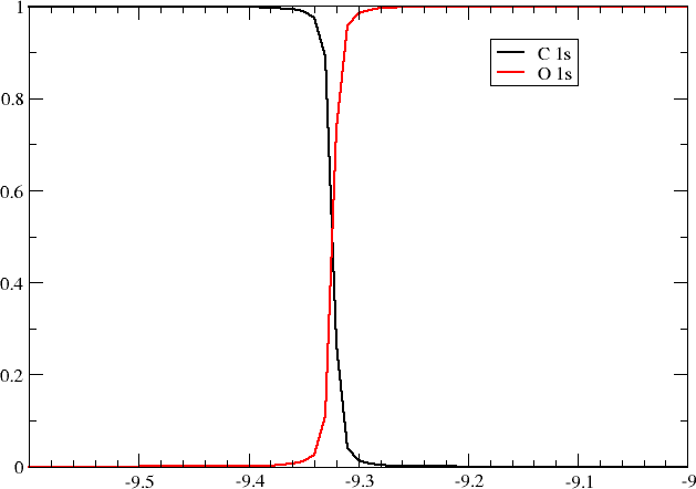
and we indeed see that the two lowest molecular orbitals now are almost degenerate with concomitant strong mixing of the \(O1s\) and \(C1s\) orbitals.
By scanning shift values in the resonance region we obtain the following plot of orbital energies of the two lowest occupied molecular orbitals
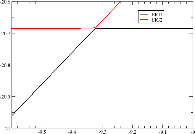
as well as the mixing of \(O1s\) and \(C1s\) orbitals in the LOMO.
At this point it may be useful to consider the diagonalization of a \(2\times2\) matrix
where eigenvalues are given by
We notably see that as we bring the two starting energies into resonance, that is \(\varepsilon_1=\varepsilon_2\), the difference \(\Delta\lambda\) becomes equal to the twice the interaction \(2|\delta|\). In this particular case \(2|\delta|=5.6\ mE_h\).
What can learn from this ? Neidig, Clark and Martin [Neidig_CoorChemRev2013] have introduced the concept of near-degeneracy driven covalency, where bonding interaction arises from near-degeneracy, even in the absence of overlap. In the above example we clearly see this mechanism at work: bringing the \(O1s\) and \(C1s\) orbitals into resonance causes strong orbital mixing. However, it would be absurd to call this bonding. The two atomic core orbitals can be disentangled by localization and we also note that their interaction is extremely weak.